Case selection with macro-level data

Comparative case studies and case selection

The comparative case study is one of the workhorse methods in political science, sociology, and partly economics. In a typical comparative case study, we study some phenomenon of interest (war, policy reforms, party strategies, economic development, etc.) in a small number of cases to figure out the underlying causes of the phenomenon (why countries go to war, why they introduce or do not introduce reforms, why they experience economic growth or stagnate, etc.). Often, the cases in a case study are countries – but this is not a requirement (Gerring 2004). Any relevant unit or action can be a case, be it court rulings (e.g., Alter and Meunier-Aitsahalia 1994; Lindstrom 2010), policy reforms (e.g., Picot 2009), or conflicts and wars (e.g., Ruane and Todd 1996) – even a comparative analysis of survey data from a small number of countries (as shown in this post) can be seen as a comparative case study where the countries are the cases.

Rules and strategies for case studies

A case study is only as good as the evidence (the newspaper articles, interviews, etc.) and the case selection strategy (a.k.a., research design) it builds on. As I explain in this other post on case selection and bullshit, the cases you choose affect the answers you get (Geddes 1990), and if you select your cases in a faulty way, you get faulty, misleading, and ultimately useless answers – you produce bullshit, whether you want to or not.

Fortunately, there are a number of different rules and strategies that you can use to select your cases in a way that minimizes the risk that your study produces flawed evidence (see e.g., Seawright and Gerring 2008; Przeworski and Teune 1970; King, Keohane, and Verba 1994; Geddes 1990; Ringdal 2018).

What not to do

Two important rules are:

1. Do not select on the dependent variable (Geddes 1990). If you want find out why countries go to war, you need to compare countries that fight wars and those who do not fight wars – you need positive and negative or high and low cases.
2. Make sure that you have enough cases. As a general rule, you need at least one more case that you have explanatory variables (King, Keohane, and Verba 1994). If you think that violent conflicts are caused by two variables, say economic deprivation and a hilly terrain (Fearon and Laitin 2003), then you need at least three comparison cases to be able to have a chance to see if this is actually true.

What do to

There are two well-known and widely used case selection strategies that help you eliminate potential alternative explanations for your phenomenon of interest (in other words, they help you avoid critical questions from pesky supervisors, examiners, or reviewers). For example, let’s say you are interested in the causes of political trust – why some citizens have high trust in politicians and political institutions and others have low trust – and you think this could be influenced by countries’ electoral systems (whether they have a proportional or majoritarian “first-past-the-post” type system). If you would now compare political trust in Sweden and the United States, you would have two countries that differ in their electoral systems – but also in many other variables (regulation of the economy, form of government, welfare state spending, etc.), and you cannot rule out that any differences in trust come from these other variables rather than the electoral systems.

A better approach would be to select two countries that are as similar as possible in all relevant aspects – except for their electoral systems. This type of case selection strategy is also called a Most-Similar-Systems-Design, or MSSD for short (Ringdal 2018, 183). Table 1 (a) below shows how this can look like: We have two cases (countries) that have different types of electoral systems but are otherwise identical in three other variables that could be relevant for political trust as well.

As a second example, let’s say you believe that people’s political trust is mainly influenced by their level of education, where trust increases with education. If you now look at this relationship only in one country (say, Norway), you open yourself up to the criticism that maybe this relationship exists only in this country and only because of Norway’s unique social and political circumstances, but the finding would not apply to other countries.

One way to address critiques like this head-on is to select cases that are as different from each other as possible. If you can show that a relationship is present in two or more cases that are very different from each other, it is likely (but not guaruanteed) that this also applies to many other cases. This case selection strategy is called a Most-Different-Systems-Design or MSDS (Ringdal 2018, 183). Table 1 (b) illustrates how such a design could look like: You pick two cases that differ in three variables that we believe are relevant, and you then ideally show that the effect of education on trust is the same in both cases. Here, we assume that the degree of female representation in politics, the political system overall, and welfare state spending could be relevant variables. (Whether that makes sense or not is a different discussion.)

Table 1: Two widely used case selection strategies

(a) Most-Similar-Systems-Design

Variable	Case A	Case B
Electoral system	Majoritarian	Proportional
Regulation	High	High
Welfare spending	Low	Low
Government	Parliamentary	Parliamentary

(b) Most-Different-Systems-Design

Variable	Case A	Case B
Female representation	High	Moderate
Political system	Const. parliamentary monarchy	Republican presidential democracy
Welfare spending	High	Low

When to use which strategy

Generally, the MSDS is best-suited if you want to show that a micro-level pattern (e.g., the effect of an individual’s education on their political trust, or gender differences) holds in very different contexts. In other words, the MSDS is a good choice if you want to control for variables that are contextual or at a higher level of analysis than the main pattern you are interested in.

The MSSD, on the other hand, is better if you want to control for other variables that are at the same level of analysis. In the example above, the main explanatory variable of interest is the electoral system – a macro-level variable – and we want to control for other macro-level variables. Here, the MSSD can help us do that.

Using R to select cases

Alright, enough with the dry theory. It is one thing to have an idea of what your case selection should theoretically look like, but you also need to actually find empirical cases and you usually also need to explain and justify your case selection in your course paper, thesis, or presentation.

This is where R and macro-level datasets like the Comparative Political Data Set (CPDS, Armingeon et al. 2024) come in handy, because you can use them to get an overview over how countries compare on many different variables, to identify countries that are either similar or different on relevant variables, and also to illustrate your selection with graphs and tables (see also this other post on how to work with macro-level datasets).

Setup

First, we need to load all relevant packages. In this case, we only need to load the tidyverse packages, and we can also already set a default theme for ggplot graphs:

library(tidyverse)

── Attaching core tidyverse packages ──────────────────────── tidyverse 2.0.0 ──
✔ dplyr     1.1.4     ✔ readr     2.1.5
✔ forcats   1.0.0     ✔ stringr   1.5.1
✔ ggplot2   3.5.2     ✔ tibble    3.2.1
✔ lubridate 1.9.4     ✔ tidyr     1.3.1
✔ purrr     1.0.4     
── Conflicts ────────────────────────────────────────── tidyverse_conflicts() ──
✖ dplyr::filter() masks stats::filter()
✖ dplyr::lag()    masks stats::lag()
ℹ Use the conflicted package (<http://conflicted.r-lib.org/>) to force all conflicts to become errors

theme_set(theme_classic())

Next, we need to download and import the CPDS dataset. Unfortunately, it is difficult to import the dataset directly into R, so we just download the Stata (.dta) version of the dataset, unpack the ZIP archive, and save the dataset somewhere where we can find it again. Then we import the saved dataset with the haven package:

cpds <- haven::read_dta("CPDS_1960_2022_Update_2024.dta")

We can then take a quick look at which countries are included:

unique(cpds$country)

 [1] "Australia"      "Austria"        "Belgium"        "Bulgaria"      
 [5] "Canada"         "Croatia"        "Cyprus"         "Czech Republic"
 [9] "Denmark"        "Estonia"        "Finland"        "France"        
[13] "Germany"        "Greece"         "Hungary"        "Iceland"       
[17] "Ireland"        "Italy"          "Japan"          "Latvia"        
[21] "Lithuania"      "Luxembourg"     "Malta"          "Netherlands"   
[25] "New Zealand"    "Norway"         "Poland"         "Portugal"      
[29] "Romania"        "Slovakia"       "Slovenia"       "Spain"         
[33] "Sweden"         "Switzerland"    "United Kingdom" "USA"           

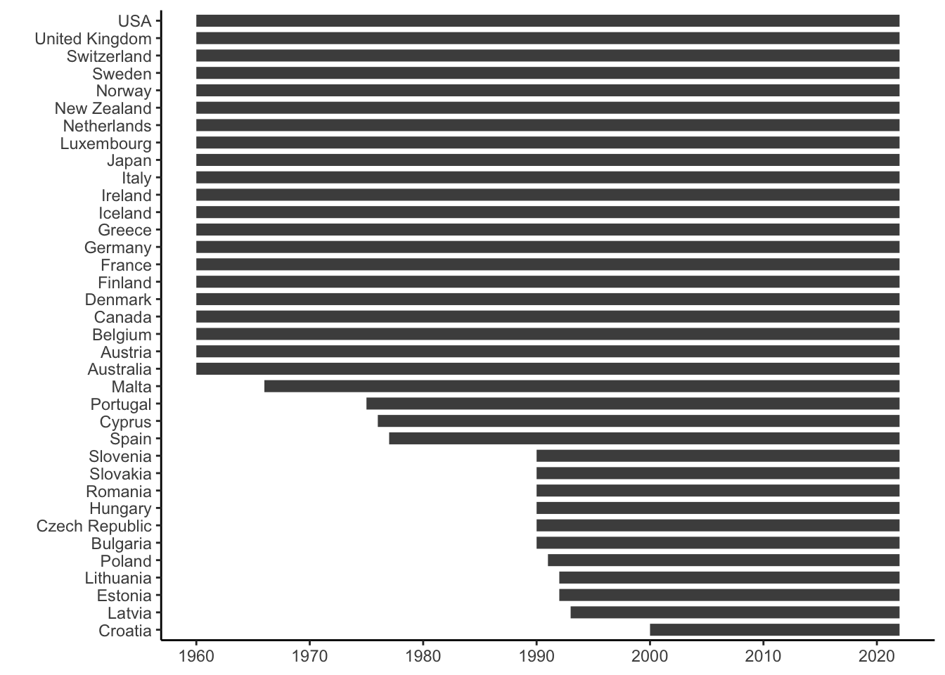
It usually also makes sense to find out for which years we have data for each country (can you make sense of this code by yourself?):¹

cpds %>% 
  group_by(country) %>% 
  summarise(start_year = min(year, na.rm = T),
            end_year = max(year, na.rm = T)) %>% 
  mutate(year_range = end_year - start_year) %>% 
 ggplot(aes(xmin = start_year, xmax = end_year, 
            y = reorder(country, year_range))) +
    geom_linerange(linewidth = 3, color = "grey30") +
    scale_x_continuous(breaks = seq(1960,2020,10)) +
    labs(y = "")

Selecting cases for an MSSD strategy

Let’s say we want to find two cases for the MSSD strategy that was described earlier, where we want different electoral systems but otherwise equality or at least similarity on all other variables.

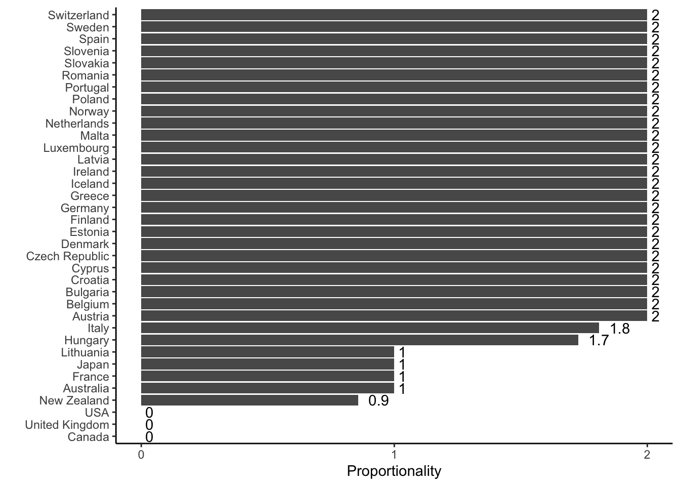
A good start is to get an overview over which countries have which type of electoral system. The CPDS contains a variable called prop (see also Huber, Ragin, and Stephens 1993), which is a categorical variable that measures whether a country has a single-member, plurality (“first-past-the-post”) electoral system (0), a modified proportional or mixed system (1), or a proportional electoral system (2).

To get this overview, we can calculate the average scores of this variable per country and visualize the result:

cpds %>% 
  group_by(country) %>% 
  summarise(mprop = mean(prop, na.rm = T)) %>% 
  ggplot(aes(x = mprop, y = reorder(country, mprop))) +
    geom_bar(stat = "identity") +
    geom_text(aes(label = round(mprop, digits = 1)), hjust = -.5) +
    scale_x_continuous(breaks = seq(0,2,1)) +
    labs(x = "Proportionality", y = "")

A clear majority of countries have proportional systems, a few have mixed systems (Lithuania, Japan, France, and Auustralia), and three countries (the USA, the UK, and Canada) have single-member “first-past-the-post” systems. Note also that a few countries (New Zealand, Italy, and Hungary) have average scores that fall between two whole numbers – which indicates that these countries changed their electoral systems at some point.

Let’s have a closer look at these countries:

cpds %>% 
  filter(country %in% c("New Zealand","Hungary","Italy")) %>% 
  ggplot(aes(x = year, y = prop)) +
    geom_line() +
    geom_point(color = "orange") +
    facet_wrap(~country, nrow = 3) +
    scale_y_continuous(breaks = seq(0,2,1)) +
    scale_x_continuous(breaks = seq(1960,2020,10)) +
    labs(x = "", y = "Proportionality")

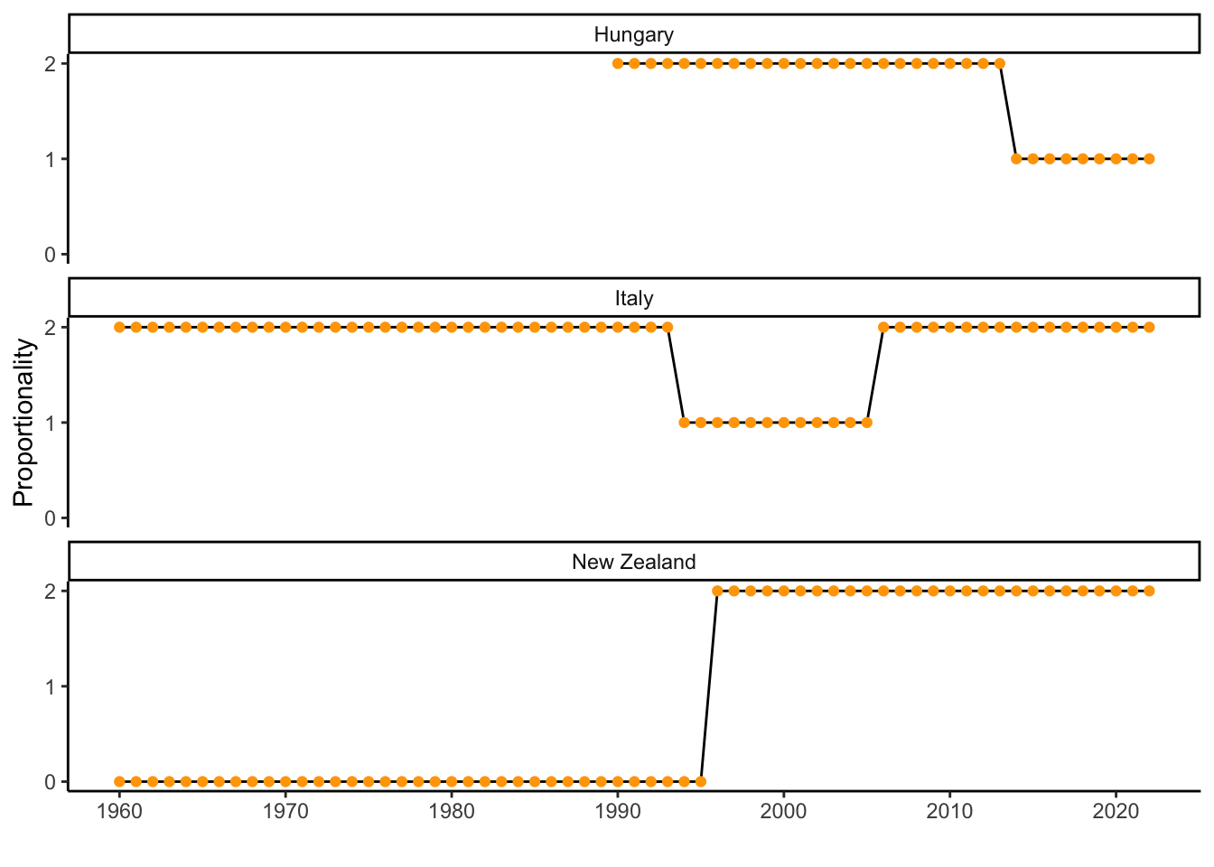
You see that Hungary went from a fully to a modified proportional system in the 2010s, Italy did the same in the 1990s but then went back to full proportionality in the 2000s, and New Zealand went from a “first-past-the-post” system to full proportionality in the mid-1990s.

One thought would be now to use this variation over time in the three countries to see if the changes in electoral rules led to changes in political trust among citizens – as long as we can assume that nothing else changed simultaneously in these countries (no changes in unemployment, economic growth, party politics, etc.), or we can control for it somehow.

An alternative would be to focus on New Zealand, which is interesting because it is the one typical English-speaking former settler colony that went away from a “first-past-the-post” system and to a proportional system, and which kept that system long enough so that its potential effects on political trust can unfold over time.

Let’s see how New Zealand compares to countries that we know are culturally and politically very similar: Australia, Canada, the United States, and the United Kingdom. To help with that, we create a variable that identifies those countries in the dataset and which we can use to highlight them in graphs:

cpds %>% 
  mutate(nzl_etal = case_match(country,
                               "New Zealand" ~ "NZL",
                               c("Canada","Australia","USA","United Kingdom") ~ "Similar",
                               .default = "Other")) -> cpds

To compare them in terms of the aspects listed in Table 1 (a) above, we can use the following variables from the CPDS:

• emprot_reg is a measure of the regulation of the labor market (see also Venn 2009)
• socexp_t_pmp is a measure of welfare state spending in relation to a country’s GDP
• pres is measure of the type of government (0 = parliamentary; 1 = semi-presidential, dominant parliament; 2 = hybrid; 3 = semi-presidential, dominant president; 4 = presidential).

The socexp_t_pmp and emprot_reg variables are generally available until 2018, so we pick that year to compare countries.

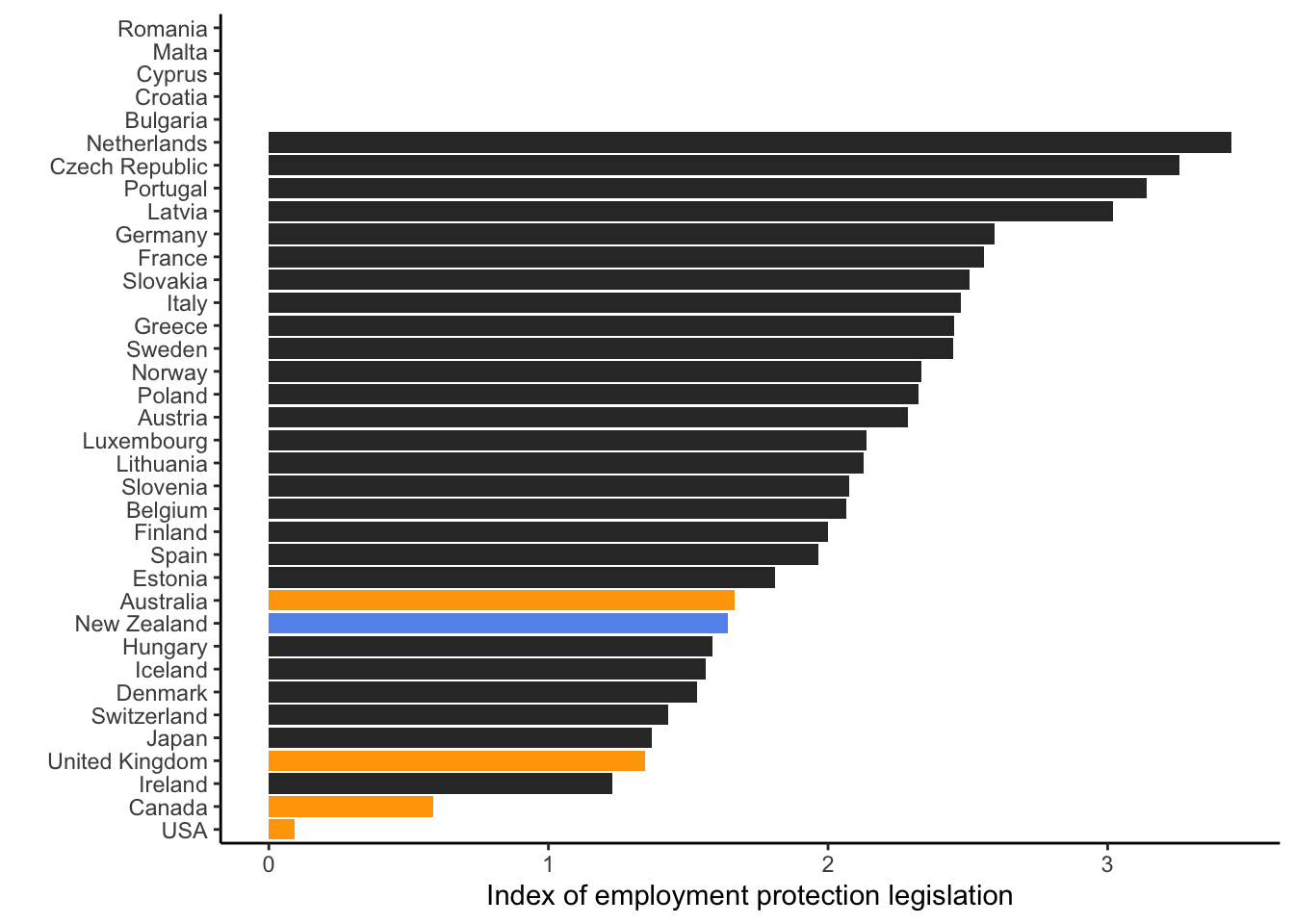
First, we look at the extent of labor market regulation:

cpds %>% 
  filter(year==2018) %>% 
  ggplot(aes(x = emprot_reg, y = reorder(country, emprot_reg), fill = nzl_etal)) +
    geom_col() +
    scale_fill_manual(values = c("NZL" = "cornflowerblue",
                                 "Similar" = "orange",
                                 "Other" = "grey20")) +
    labs(y = "", x = "Index of employment protection legislation") +
    theme(legend.position = "none")

Warning: Removed 5 rows containing missing values or values outside the scale range
(`geom_col()`).

New Zealand and Australia stand a bit apart from the other English-speaking countries, but are very similar to each other.

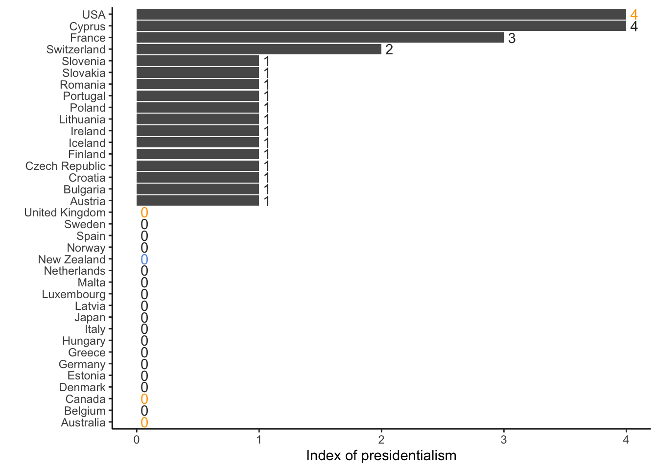
Next, we look at the type of government:

cpds %>% 
  filter(year==2018) %>% 
  ggplot(aes(x = pres, y = reorder(country, pres))) +
    geom_col() +
    geom_text(aes(label = pres, color = nzl_etal), hjust = -.5) +
    scale_color_manual(values = c("NZL" = "cornflowerblue",
                                 "Similar" = "orange",
                                 "Other" = "grey20")) +
    labs(y = "", x = "Index of presidentialism") +
    theme(legend.position = "none")

Both Australia and New Zealand are clearly parliamentary democracies, very unlike the US.

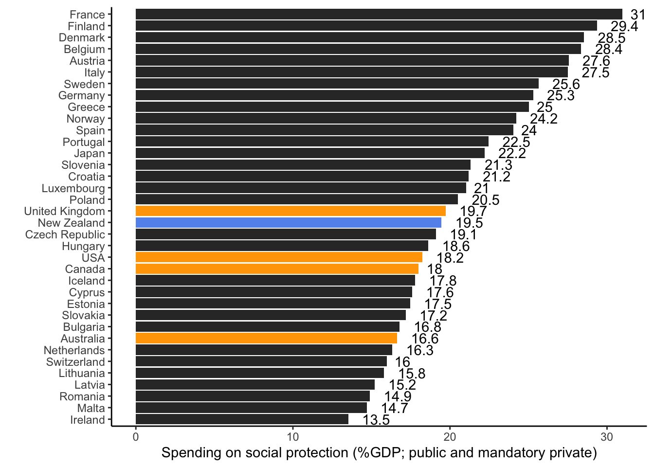
Finally, let’s have a look at how countries compare in terms of welfare state spending:

cpds %>% 
  filter(year==2018) %>% 
  ggplot(aes(x = socexp_t_pmp, y = reorder(country, socexp_t_pmp), fill = nzl_etal)) +
    geom_col() +
    geom_text(aes(label = round(socexp_t_pmp, digits = 1)), hjust = -.5) +
    scale_fill_manual(values = c("NZL" = "cornflowerblue",
                                 "Similar" = "orange",
                                 "Other" = "grey20")) +
    labs(y = "", x = "Spending on social protection (%GDP; public and mandatory private)") +
    theme(legend.position = "none")

Here, New Zealand is more similar to the United Kingdom than to Australia, but the two countries are not very far apart. Also, many would say that welfare state spending is “epiphenomenal” (Esping-Andersen 1990) anyways and that a look at the underlying rules and institutions reveals that Australia and New Zealand both belong to the liberal welfare state regime (see also Castles 1993).

So, at least in the late 2010s, Australia and New Zealand are two countries that are historically, politically, and economically very similar – but differ in their electoral systems. This could be a potential MSSD case selection that we can explain and defend with evidence.

Selecting cases for an MDSD strategy

The workflow to select potential cases for an MDSD strategy is basically the same as that shown above for an MSSD strategy: We sift through and visualize relevant macro-level data to see how potential cases compare. The only difference is that we look for differences rather than similarities in the case of an MDSD.

As per Table 1 (b), we want to find two cases that are as different as possible in terms of their political systems, female representation, and welfare state spending (the variables which we assume to be relevant, for the sake of illustration).

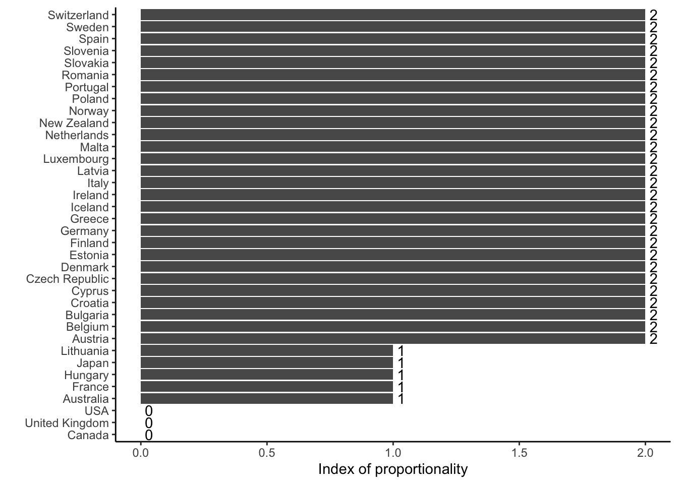
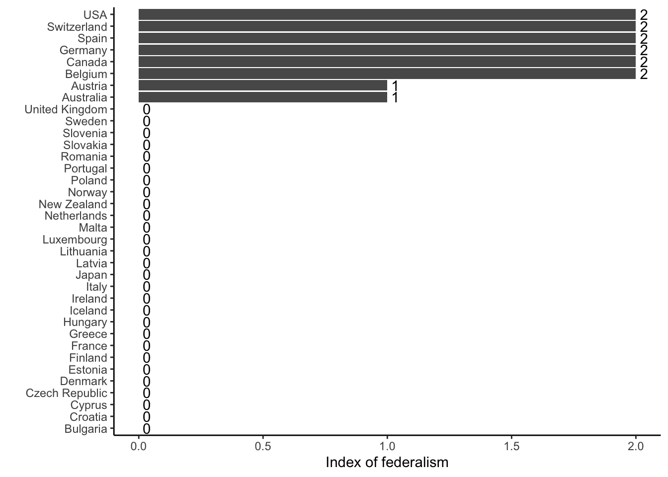
To identify cases – countries – that differ in terms of their political systems, we can again use data from the CPDS, specifically the variables measuring the structure of political institutions in a given country like the prop and pres variables used above. A third one we could consider is called fed and measures the degree of federalism in a country (0 = no; 1 = weak; 2 = strong). To keep things simple, we look again at data from 2018, but this is something you can of course adapt in your own analysis.

cpds %>% 
  filter(year == 2018) %>% 
  ggplot(aes(x = prop, y = reorder(country, prop))) +
    geom_col() +
    geom_text(aes(label = prop), hjust = -.5) +
    labs(y = "", x = "Index of proportionality") +
    theme(legend.position = "none")

If we take Norway (the case we started from earlier) as a baseline, then the three countries with “first-past-the-post” electoral systems are very different from it. The US are in addition also the one democracy out of the three with “first-past-the-post” systems that does not have a monarch as its head of state.

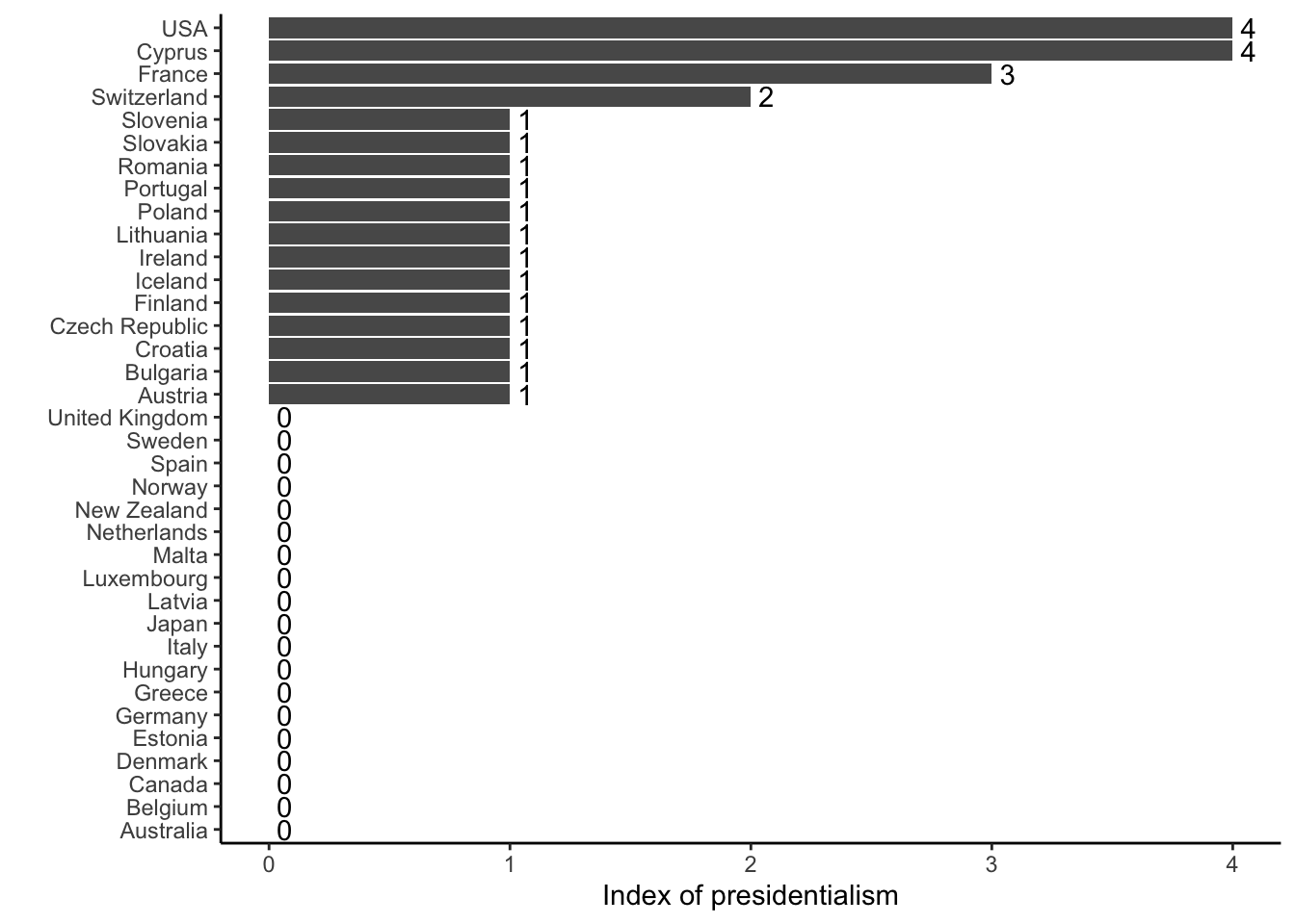
cpds %>% 
  filter(year == 2018) %>% 
  ggplot(aes(x = pres, y = reorder(country, pres))) +
    geom_col() +
    geom_text(aes(label = pres), hjust = -.5) +
    labs(y = "", x = "Index of presidentialism") +
    theme(legend.position = "none")

When we look at the degree of presidentialism, the US and Norway are clearly worlds apart.

cpds %>% 
  filter(year == 2018) %>% 
  ggplot(aes(x = fed, y = reorder(country, fed))) +
    geom_col() +
    geom_text(aes(label = fed), hjust = -.5) +
    labs(y = "", x = "Index of federalism") +
    theme(legend.position = "none")

This is the same when we look at the degree of federalism.

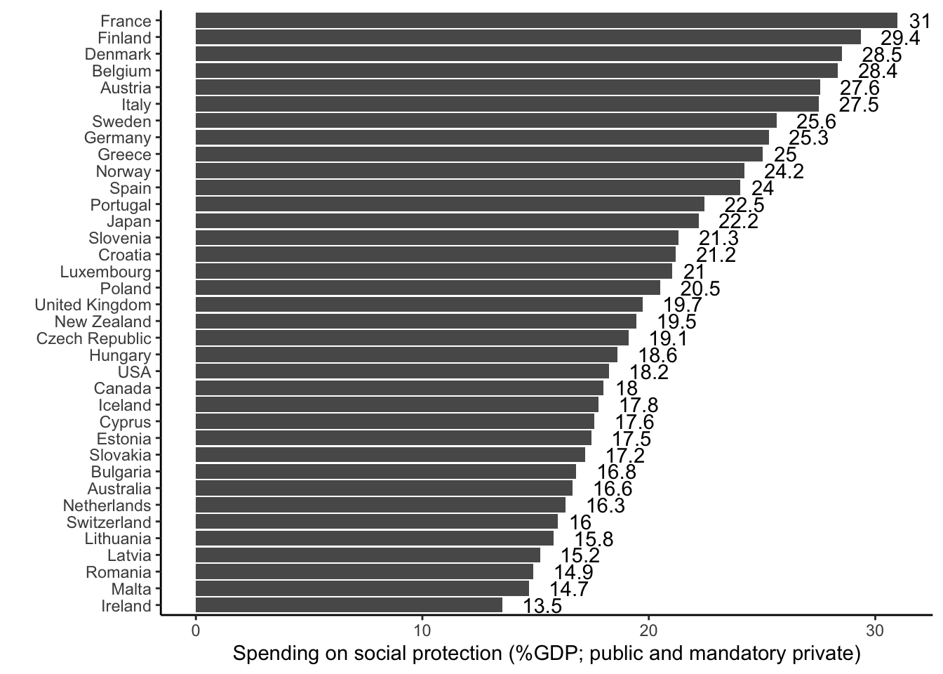
cpds %>% 
  filter(year==2018) %>% 
  ggplot(aes(x = socexp_t_pmp, y = reorder(country, socexp_t_pmp))) +
    geom_col() +
    geom_text(aes(label = round(socexp_t_pmp, digits = 1)), hjust = -.5) +
    labs(y = "", x = "Spending on social protection (%GDP; public and mandatory private)") +
    theme(legend.position = "none")

The US are roughly in the middle of the pack when it comes to welfare state spending, but score lower than Norway. And, again, a look at Esping-Andersen (1990) would suggest that the two countries are very different when it comes to the policies and institutions that are underneath the spending figures.

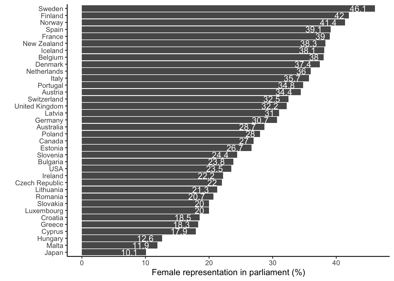
Now to the final aspect, female representation in politics. Here, we can use the womenpar variable from the CPDS, which measures the percentage of seats in parliament that are held by women (regardless of their partisan affiliation). As before, this variable is available until 2018:

cpds %>% 
  filter(year == 2018) %>% 
  ggplot(aes(x = womenpar, y = reorder(country, womenpar))) +
    geom_col() +
    geom_text(aes(label = round(womenpar, digits = 1)), hjust = 1.5, color = "white") +
    labs(y = "", x = "Female representation in parliament (%)") +
    theme(legend.position = "none")

Once again, Norway and the US are quite far apart. Norway, along with Sweden and Finland, is one of the top scorers when it comes to gender equality in politics, while the US are in the bottom half.

Overall, if you would analyze survey data from Norway and the US (e.g., from the International Social Survey Project) to see if education has an effect on political trust and if you find (roughly) the same effect in both cases, then you have a strong counterargument to potential criticism that your findings might not apply to other contexts. If it works in the US and Norway, two very different countries and societies, then it likely also works in many other contexts.

Next steps

This post showed how you can use macro-level data to select cases for a comparative case study, focusing on countries as cases.

Obviously, and as mentioned above, countries are not the only units that can be potential cases – regions, parties, interest groups, court rulings, or wars and conflicts can also be cases that can be compared. In addition, you would of course think more carefully about the variables you need to look at in a real analysis (theory is your friend here!), and this might mean that you have to look at several different datasets to get a complete picture of how your cases compare on those variables. Still, the fundamental logic – exploring data to identify relevant cases – also applies to those situations, you would only use different datasets (see e.g., this post for a list).

The techniques we used here for also relatively simple and purely descriptive, and there are of course also more advanced methods to select cases based on a quantitative analysis for a more detailed and in-depth qualitative investigation. Seawright & Gerring (2008) show how to do that.

References

Alter, Karen J, and Sophie Meunier-Aitsahalia. 1994. “Judicial Politics in the European Community: European Integration and the Pathbreaking Cassis de Dijon Decision.” Comparative Political Studies 26 (4): 535–61.

Armingeon, Klaus, Sarah Engler, Lucas Leemann, and David Weisstanner. 2024. Comparative Political Data Set 1960-2022. Zurich, Lueneburg, & Lucerne: University of Zurich, Leuphana University Lueneburg,; University of Lucerne.

Castles, Francis G., ed. 1993. Families of Nations: Patterns of Public Policy in Western Democracies. Aldershot: Dartmouth Publishing Co.

Esping-Andersen, Gøsta. 1990. The Three Worlds of Welfare Capitalism. Cambridge: Polity Press.

Fearon, James D., and David D. Laitin. 2003. “Ethnicity, Insurgency, and Civil War.” American Political Science Review 97 (1): 75–90.

Geddes, Barbara. 1990. “How the Cases You Choose Affect the Answers You Get: Selection Bias in Comparative Politics.” Political Analysis 2 (1): 131–50.

Gerring, John. 2004. “What Is a Case Study and What Is It Good For?” American Political Science Review 98 (2): 341–54.

Huber, Evelyne, Charles Ragin, and John D. Stephens. 1993. “Social Democracy, Christian Democracy, Constitutional Structure, and the Welfare State.” American Journal of Sociology 99 (3): 711–49.

King, Gary, Robert O. Keohane, and Sidney Verba. 1994. Designing Social Inquiry. Scientific Inference in Qualitative Research. Princeton: Princeton University Press.

Lindstrom, Nicole. 2010. “Service Liberalization in the Enlarged EU: A Race to the Bottom or the Emergence of Transnational Political Conflict?” Journal of Common Market Studies 48 (5): 1307–27.

Picot, Georg. 2009. “Party Competition and Reforms of Unemployment Benefits in Germany: How a Small Change in Electoral Demand Can Make a Big Difference.” German Politics 18 (2): 155–79.

Przeworski, Adam, and Henry Teune. 1970. The Logic of Comparative Social Inquiry. New York: Wiley.

Ringdal, Kristen. 2018. Enhet Og Mangfold: Samfunnsvitenskapelig Forskning Og Kvantitativ Metode. 4. ed. Bergen: Fagbokforlaget.

Ruane, Joseph, and Jennifer Todd. 1996. The Dynamics of Conflict in Northern Ireland: Power, Conflict and Emancipation. Cambridge: Cambridge University Press.

Seawright, Jason, and John Gerring. 2008. “Case Selection Techniques in Case Study Research.” Political Research Quarterly 61 (2): 294–308.

Venn, Danielle. 2009. “Legislation, Collective Bargaining and Enforcement: Updating the OECD Employment Protection Indicators.” OECD Social, Employment and Migration Working Papers 89.

Footnotes

1. To explain: We group the data by country and then let R figure out the start (min) and end (max) year per country within summarize(). Based on that result, we calculate the difference between start and end as year_range. Next, we visualize the result with ggplot, where we order the countries on the x-axis according to how many years we have data for and use geom_linerange() to indicate the time period for which a given country is covered in the dataset.