library(tidyverse)
library(texreg)Are people influenced by the environments they live in?
Are people’s opinions, behaviors, or perceptions affected by the environments (or “macro-level contexts”) they live in? Social and economic scientists often argue that this is indeed the case. For example, many sociologists argue that societal norms shape people’s behavior (e.g., that men do more of the housework in societies with egalitarian gender norms), and political scientists similarly suggest that political institutions influence political attitudes and behavior (e.g., that people participate more in elections in proportional or majoritarian electoral systems).
Obviously, these theories are only as good as the evidence in support of them. To test these types of theories, one needs to compare people’s opinions or behavior across contexts with different social norms, political institutions, or other macro-level factors that might have an influence on people. This is usually done with comparative survey data such as data from the European Social Survey, the International Social Survey Program, the Eurobarometer, the OECD Risks that Matter survey, or the World Values Study.1 The big advantage that comparative survey data offer is that they are standardized: The same survey with the exact same questions is conducted in multiple countries at the same time, so that people’s responses to the questions – i.e., their attitudes or behavior – can be directly compared.2 This means that one can use these survey data to find out how macro-level environmental factors influence patterns at the micro-level.
Working with cross-country comparative survey data can seem daunting to students who have only learned about relatively simple methods (linear regression, graphical analyses), and it really is objectively a relatively complicated type of methods with lots of snags and pitfalls (see e.g., Stegmueller 2013; Bryan and Jenkins 2016; Elff et al. 2021; Fairbrother 2014; Schmidt-Catran et al. 2019; Steenbergen and Jones 2002). However, as always in life, there are easier and more complicated ways of doing this.
This post shows you how to do this type of analysis in the easiest way possible, using R, data from the European Social Survey, and techniques that undergraduate students usually learn in their introductory statistics courses: Descriptive statistics and linear regression models (following Blekesaune and Bjørkhaug 2021).
TipThe method in a nutshell (TL;DR)
- You pick a cross-country survey dataset (e.g., from the European Social Survey, the World Values Survey, the International Social Survey Program, or the Euro-, Afro-, or Arabbarometer) that contains relevant variables/questions for multiple countries that could be relevant to compare.
- Out of the countries that are covered in your survey dataset, you select a small number (at least two and up to four or five) countries that differ in relevant ways in relevant macro-level aspects (e.g., one has overall traditional gender norms, the other is very progressive) but are otherwise as similar as possible so that you can rule out as many alternative explanations as possible.3
- You analyze the data from each of the countries separately using standard techniques (e.g., graphs, statistical tests, linear regression), but…
- You present the results from each country together so that you can see similarities and differences in relevant patterns (e.g., gender differences in household work or political attitudes).
Thematically, we look at the effect of gender (a micro-level variable) on political opinions (another micro-level attitude) and how that effect is influenced by countries’ economic structures (a macro-level variable). Simply put, we ask: are men and women more or less politically divided in their political opinions depending on the economic environment they live in (Inglehart and Norris 2000; Iversen and Rosenbluth 2010, 2006)? In yet other words, we do a simple re-test of the “household bargaining theory” of political gender differences by Iversen & Rosenbluth (2006, 2010).
The Iversen/Rosenbluth hypothesis in the smallest of nutshells
Very (very) simply put, Iversen & Rosenbluth (2006, 2010) argue that women are politically to the left of men, other things equal, but also that the size of this gap – how far apart women and men are – depends on macro-level factors such as how countries’ economies are structured. In countries that have economies that rely strongly on specific skills (think: highly trained craftsmen and -women that are really good at a few specific tasks), this gap should be particularly large. In contrast, in countries that rely more on general skills (think: flexible professionals that can quickly switch between jobs), women and men should be more equal in their political opinions.
Re-analysis using ESS data
We do a new test of this hypothesis using data from the tenth (2018) round of the European Social Survey (ESS).
Out of all the countries covered by this round of the ESS, we select the following two countries based on qualitative information we have from Iversen & Rosenbluth (2006), but also other studies (Hall and Soskice 2001; Iversen and Soskice 2001):
- Ireland, which is known to rely strongly on general skills. Here, we expect a small gender gap.
- Norway, which relies on specific skills. Here, we expect a large gender gap.
Ideally, one would pick countries that are as similar as possible except for the structure of their economy so that we can really isolate the effect of that one factor (see also above), but we keep things simple and convenient for now and stick with Norway and Ireland.
We use the following micro-level variables from the ESS:
- Left-right ideology (
lrscale). This is measures people’s general political orientation and is the dependent variable. - Gender (
gndr; male/female). This is the central independent variable here. - Household income (
hinctnta): This is a relevant control variable. - Age (
agea; years): Also a control variable. - Education (
eduyrs): A final variable we want to control for.
Packages
We use the tidyverse for data management & visualization and texreg to present regression results:
Set theme for graphs
The classic theme just looks better…
theme_set(theme_classic())Data import
You can download the data for free (after a registration) from https://www.europeansocialsurvey.org/. I use the .dta (Stata) version and saved the dataset as ESS10.dta on my computer. I use the haven package to import the dataset, and then immediately convert the dataset to the traditional R format with labelled::unlabelled (to be able to do this, you need to have both of these packages installed. Loading them with library() is not necessary).
ess <- labelled::unlabelled(haven::read_dta("ESS10.dta"))Trimming
The entire ESS is massive. To make things easier to handle, we select only the relevant variables (plus some useful “administrative” ones such as idno, essround, and cntry):
ess %>%
  select(idno,essround,cntry,lrscale,gndr,agea,eduyrs,hinctnta) -> ess
Data cleaning
Household income (hinctnta) and left-right self-placement (lrscale) are factors and need to be correctly converted to numeric before we can use them in a regression analysis:
class(ess$hinctnta)[1] "factor"class(ess$lrscale)[1] "factor"bst290::visfactor(dataset = ess,
variable = "hinctnta") # no label/value divergence, no adjustment needed values labels
1 J - 1st decile
2 R - 2nd decile
3 C - 3rd decile
4 M - 4th decile
5 F - 5th decile
6 S - 6th decile
7 K - 7th decile
8 P - 8th decile
9 D - 9th decile
10 H - 10th decilebst290::visfactor(dataset = ess,
variable = "lrscale") # labels/values are off by 1, needs to be adjusted values labels
1 Left
2 1
3 2
4 3
5 4
6 5
7 6
8 7
9 8
10 9
11 Rightess %>%
mutate(hhinc = as.numeric(hinctnta),
lrscale = as.numeric(lrscale) - 1) -> essCountry selection
The final “trimming” operation we need to do is to select only the two countries we want to compare. This is easy to do with filter(), and we create separate datasets for each of the two countries:
unique(ess$cntry) [1] "BE" "BG" "CH" "CZ" "EE" "FI" "FR" "GB" "GR" "HR" "HU" "IE" "IS" "IT" "LT"
[16] "ME" "MK" "NL" "NO" "PT" "SI" "SK"ess %>%
filter(cntry=="NO") -> norway
ess %>%
filter(cntry=="IE") -> irelandDescriptive analysis of political gender gaps by country
It is good practice to first do a bit of visual analysis to get a sense of how the data look before moving to more complicated statistical analyses. Here, we use a bit of dplyr (group_by() & summarize()) to calculate the political gender gap in each country – how men and women differ, on average, in their ideology – and then visualize the result with a ggplot() bar graph.
ireland %>%
  group_by(gndr) %>%
  summarise(avg_lr = mean(lrscale, na.rm = T)) %>%
  ggplot(aes(x = gndr, y = avg_lr)) +
    geom_bar(stat = "identity") +
    geom_text(aes(label = round(avg_lr, digits = 1)), vjust = -.5) +
    scale_y_continuous(limits = c(0,6)) +
    labs(x = "Gender", y = "Average left-right placement",
         caption = "Higher scores = more conservative",
         title = "Ireland")
norway %>%
  group_by(gndr) %>%
  summarise(avg_lr = mean(lrscale, na.rm = T)) %>%
  ggplot(aes(x = gndr, y = avg_lr)) +
    geom_bar(stat = "identity") +
    geom_text(aes(label = round(avg_lr, digits = 1)), vjust = -.5) +
    scale_y_continuous(limits = c(0,6)) +
    labs(x = "Gender", y = "Average left-right placement",
         caption = "Higher scores = more conservative",
         title = "Norway")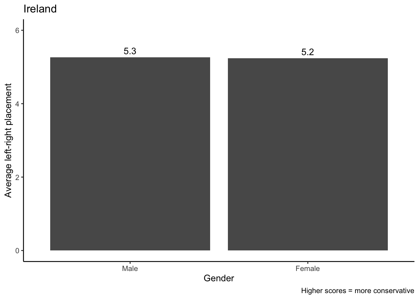
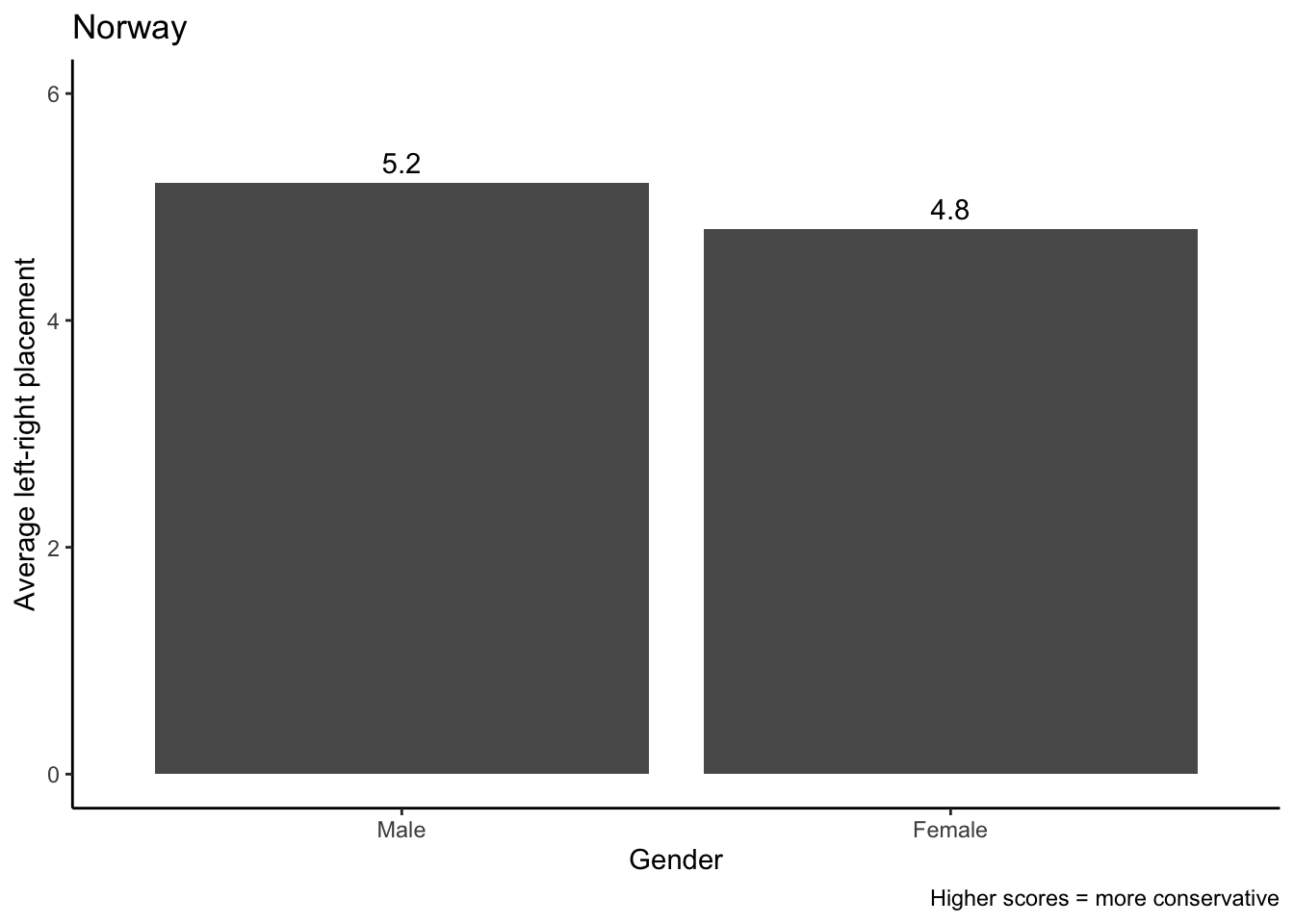
It looks like the data support the hypothesis. We expected a small ideological gap between men and women in Ireland, and that is what we find: Men and women hardly differ on average in their left-right orientation (5.3 - 5.2 = 0.1). In contrast, this difference is four times as large (5.2 - 4.8 = 0.4), which is what we would have expected.
Regression analysis
While the visual analysis is useful, we also need to do a more thorough test where we control for other variables. To do that, we do a simple linear (OLS) regression analysis separately for each country:
# Baseline model
no_mod1 <- lm(lrscale ~ gndr,
               data = norway)

# With controls
no_mod2 <- lm(lrscale ~ gndr + agea + eduyrs + hhinc,
               data = norway)

# Baseline model
ie_mod1 <- lm(lrscale ~ gndr,
               data = ireland)

# With controls
ie_mod2 <- lm(lrscale ~ gndr + agea + eduyrs + hhinc,
               data = ireland)
We use screenreg() from the texreg package to show the results directly next to each other so that we can spot differences between the two countries more easily:
screenreg(list(no_mod1,no_mod2,ie_mod1,ie_mod2),
          stars = 0.05,
          custom.header = list("Norway" = 1:2, "Ireland" = 3:4),
          custom.model.names = c("No controls","Controls",
                                 "No controls","Controls"),
          custom.coef.map = list("(Intercept)" = "Intercept",
                                 "gndrFemale" = "Female",
                                 "agea" = "Age",
                                 "eduyrs" = "Education (years)",
                                 "hhinc" = "Household income (deciles)"))
=========================================================================
                                    Norway                 Ireland
                            ----------------------  ---------------------
                            No controls  Controls   No controls  Controls
-------------------------------------------------------------------------
Intercept                      5.21 *       5.41 *     5.26 *      4.61 *
                              (0.09)       (0.35)     (0.08)      (0.38)
Female                        -0.41 *      -0.38 *    -0.02       -0.03
                              (0.13)       (0.13)     (0.11)      (0.13)
Age                                         0.01 *                 0.02 *
                                           (0.00)                 (0.00)
Education (years)                          -0.10 *                -0.01
                                           (0.02)                 (0.02)
Household income (deciles)                  0.12 *                -0.03
                                           (0.03)                 (0.03)
-------------------------------------------------------------------------
R^2                            0.01         0.04       0.00        0.03
Adj. R^2                       0.01         0.04      -0.00        0.02
Num. obs.                   1375         1300       1516         993
=========================================================================
* p < 0.05
Women are again significantly more to the left than men in Norway but not in Ireland – which is what Iversen & Rosenbluth would have predicted. These effects are barely affected by the inclusion of controls for age, education, and household income.
Overall, this relatively simple re-test supports the Iversen/Rosenbluth theory of gender differences.
Next steps
You have now seen how you can do a simple cross-country comparative analysis of survey data with R. Obviously, you can adapt this type of analysis to many different questions so long as you have relevant data. For example, if you have macro-level indicators of how countries’ electoral systems look like (which you do: https://cpds-data.org/) and comparative survey data on people’s electoral behavior (which you can get via the ESS), you can test if rates of participation in election differ between types of electoral systems. The same applies to any combination of macro-level factor and micro-level behavior you can think of and have data for.
Importantly, you may also have noticed that we did not use any form of quantitative data to measure macro-level factors or to pick countries – we simply relied on findings from other studies to select relevant countries.
Finally, there are obviously ways to make this type of analysis more sophisticated. One additional step one can take is to test statistically if the coefficients from regression models are statistically significantly different from each other. Paternoster et al. (1998) have developed a simple formula for this that works basically like a standard two-sample t-test.
The most advanced way to compare survey data from different countries is obviously with a multi-level or hierarchical regression analysis. This is what academic researchers usally use because it multi-level regression models make it possible to use all available data from a comparative survey dataset instead of picking only a small number of countries. This makes it possible to estimate more complicated models and to get more accurate and reliable results. If you want to learn more about this, there is a series of articles that explains these models in a very intuitive and easy fashion (Merlo, Yang, et al. 2005; Merlo, Chaix, et al. 2005a, 2005b; Merlo et al. 2006; see also Steenbergen and Jones 2002), and the book by Finch et al. (2014) explains how you implement these models in R.
References
Blekesaune, Arild, and Hilde Bjørkhaug. 2021. “Analyser av surveydata 2: Logistiske regresjonsmodeller og sammenligning av data fra flere land.” In En smak av forskning: Bacheloroppgaven som prosjekt, prosess og produkt, edited by Ingvill Stuvøy, Gunhild Tøndel, and Aksel Tjora. Cappelen Damm Akademisk.
Bryan, Mark L., and Stephen P. Jenkins. 2016. “Multilevel Modelling of Country Effects: A Cautionary Tale.” European Sociological Review 32 (1): 3–22.
Elff, Martin, Jan Paul Heisig, Merlin Schaeffer, and Susumu Shikano. 2021. “Multilevel Analysis with Few Clusters: Improving Likelihood-Based Methods to Provide Unbiased Estimates and Accurate Inference.” British Journal of Political Science 51 (1): 412–26.
Fairbrother, Malcolm. 2014. “Two Multilevel Modeling Techniques for Analyzing Comparative Longitudinal Survey Datasets.” Political Science Research and Methods 2 (1): 119–40.
Finch, W Holmes, Jocelyn E Bolin, and Ken Kelley. 2014. Multilevel Modeling Using r. CRC Press.
Hall, Peter A., and David Soskice, eds. 2001. Varieties of Capitalism: The Institutional Foundations of Comparative Advantage. Oxford University Press.
Inglehart, Ronald, and Pippa Norris. 2000. “The Developmental Theory of the Gender Gap: Women’s and Men’s Voting Behavior in Global Perspective.” International Political Science Review 21 (4): 441–63.
Iversen, Torben, and Frances Rosenbluth. 2006. “The Political Economy of Gender: Explaining Cross-National Variation in the Gender Division of Labor and the Gender Voting Gap.” American Journal of Political Science 50 (1): 1–19.
Iversen, Torben, and Frances Rosenbluth. 2010. Women, Work, & Politics: The Political Economy of Gender Inequality. Yale University Press.
Iversen, Torben, and David Soskice. 2001. “An Asset Theory of Social Policy Preferences.” American Political Science Review 95 (4): 875–93.
King, Gary, Robert O. Keohane, and Sidney Verba. 1994. Designing Social Inquiry. Scientific Inference in Qualitative Research. Princeton University Press.
Landman, Todd. 2003. Issues and Methods in Comparative Politics: An Introduction. 2nd ed. Routledge.
Merlo, Juan, Basile Chaix, Henrik Olsson, et al. 2006. “A Brief Conceptual Tutorial of Multilevel Analysis in Social Epidemiology: Using Measures of Clustering in Multilevel Logistic Regression to Investigate Contextual Phenomena.” Journal of Epidemiology and Community Health 60 (4): 290–97.
Merlo, Juan, Basile Chaix, Min Yang, John Lynch, and Lennart Råstam. 2005a. “A Brief Conceptual Tutorial on Multilevel Analysis in Social Epidemiology: Interpreting Neighbourhood Differences and the Effect of Neighbourhood Characteristics on Individual Health.” Journal of Epidemiology and Community Health 59 (12): 1022–29.
Merlo, Juan, Basile Chaix, Min Yang, John Lynch, and Lennart Råstam. 2005b. “A Brief Conceptual Tutorial on Multilevel Analysis in Social Epidemiology: Linking the Statistical Concept of Clustering to the Idea of Contextual Phenomenon.” Journal of Epidemiology and Community Health 59 (6): 443–49.
Merlo, Juan, Min Yang, Basile Chaix, John Lynch, and Lennart Råstam. 2005. “A Brief Conceptual Tutorial on Multilevel Analysis in Social Epidemiology: Investigating Contextual Phenomena in Different Groups of People.” Journal of Epidemiology and Community Health 59 (9): 729–36.
Paternoster, Raymond, Robert Brame, Paul Mazerolle, and Alex Piquero. 1998. “Using the Correct Statistical Test for the Equality of Regression Coefficients.” Criminology 36 (4): 859–66.
Ringdal, Kristen. 2018. Enhet Og Mangfold: Samfunnsvitenskapelig Forskning Og Kvantitativ Metode. 4. Fagbokforlaget.
Schmidt-Catran, Alexander W, Malcolm Fairbrother, and Hans-Jürgen Andreß. 2019. “Multilevel Models for the Analysis of Comparative Survey Data: Common Problems and Some Solutions.” Kölner Zeitschrift für Soziologie & Sozialpsychologie 71 (Suppl 1): 99–128.
Steenbergen, Marco R., and Bradford S. Jones. 2002. “Modeling Multilevel Data Structures.” American Journal of Political Science 46 (1): 218–37.
Stegmueller, Daniel. 2013. “How Many Countries for Multilevel Modeling? A Comparison of Frequentist and Bayesian Approaches.” American Journal of Political Science 57 (3): 748–61.
Footnotes
See https://github.com/erikgahner/PolData?tab=readme-ov-file#cross-sectional for a list of comparative survey data projects.↩︎
Obviously, questionnaires are translated where languages differ, and there are sometimes cases where some questions are only asked in a subset of all countries that are included in a given survey.↩︎
See also Ringdal (2018), Chapter 9, King et al. (1994), or Landman (2003), Chapters 2-3 for an explanation of relevant case selection strategies↩︎
Citation
BibTeX citation:
@online{knotz2025,
  author = {Knotz, Carlo},
  title = {Comparing People’s Behavior and Attitudes Across Countries},
  date = {2025-03-08},
  url = {https://cknotz.github.io/getstuffdone_blog/posts/compa_survey/},
  langid = {en}
}
For attribution, please cite this work as:
Knotz, Carlo. 2025. “Comparing People’s Behavior and Attitudes
Across Countries.” March 8. https://cknotz.github.io/getstuffdone_blog/posts/compa_survey/.