How vulnerable are workers to globalization (and what effects does this have)?

Survey data
Globalization
Merging data
ESS
Political science
Sociology
Economics
Author

Carlo Knotz

Published

March 10, 2025

The losers of globalization and trade

‘Globalization destroys jobs’ or similar statements are often made by politicians or business and labor leaders, especially when new trade agreements are in the process of being negotiated. And indeed, even though free trade is generally beneficial to countries’ economies as a whole, there are usually some workers who are negatively affected by increased competition from abroad (Autor, Dorn, and Hanson 2013; Heckscher 1919; Ohlin 1933). These negative economic effects can then also have further political and social effects, for example in the form of increased demands for social protection (Walter 2010), increased political polarization and conflict (Autor et al. 2020), and rising rates of divorce and out-of-wedlock births (Anelli, Giuntella, and Stella 2024).

To be able to study these (and potentially other) effects, researchers obviously need some of measurement of how exposed and vulnerable workers are to the negative effects of trade and international competition. One way to measure this is with indicators of ‘offshoreability’ — how easy or difficult is it to move the work done by people in different occupations to other countries? Different such indicators have been developed, but one that is relatively widely used are the indicators of offshoreability by Blinder & Krueger (2013). They use a survey-based approach, where they ask workers about their perceptions of how easy it would be to move their jobs abroad and confirm this with a second survey of experts.

The rest of this post will show you how you can access the data, import them into R, and merge them with data from round 7 (2014) of the European Social Survey so that you can analyze how vulnerability to globalization affects people’s attitudes and behavior.

Accessing the data

Luckily, the Blinder/Krueger data are publicly available as part of the replication data package of a second (important) research article, which compares the effects of globalization and technological change on workers (Goos, Manning, and Salomons 2014). Goos et al. have archived the research data they use in the ICPSR Data Archive: https://doi.org/10.3886/E112846V1. There, under Data, is the task.dta dataset, which contains the offshoreability scores and, as a bonus, also additional scores on how exposed workers are to losing their jobs to robots and other automated technology Thewissen and Rueda (2019). You can download the dataset for free, after a quick login.

Importing and merging the data with ESS data

Preparation

Merging the data with ESS survey data is not as difficult as it might seem. The first step is to make sure that you also have access to ESS data (which can be downloaded for free from europeansocialsurvey.org), and that both datasets are stored in your current working directly (“folder”) so that R can directly find and import them. As mentioned above, the example here uses data from the 7th ESS round, so if you do not already have the data on your computer, quickly download them (in Stata/.dta format).

In R, we first load the tidyverse because it contains functions that we need to be able to work with and visualize the data. I am also setting the ggplot theme to classic:

library(tidyverse)
── Attaching core tidyverse packages ──────────────────────── tidyverse 2.0.0 ──
✔ dplyr     1.1.4     ✔ readr     2.1.5
✔ forcats   1.0.0     ✔ stringr   1.5.1
✔ ggplot2   3.5.1     ✔ tibble    3.2.1
✔ lubridate 1.9.4     ✔ tidyr     1.3.1
✔ purrr     1.0.4     
── Conflicts ────────────────────────────────────────── tidyverse_conflicts() ──
✖ dplyr::filter() masks stats::filter()
✖ dplyr::lag()    masks stats::lag()
ℹ Use the conflicted package (<http://conflicted.r-lib.org/>) to force all conflicts to become errors
theme_set(theme_classic())

Data import

Then we first import the ESS dataset with haven:

ess7 <- haven::read_dta("ess7.dta")

The ESS is quite big, so to make things easier we select only a few variables that we want to work with:

ess7 %>% 
  select(idno,cntry,essround,isco08,gndr,agea,trstplt) -> ess7
  • idno and essround are “administrative” variables that are always good to keep
  • cntry designates which country a given respondent comes from, and this one should always be kept
  • isco08 is the respondents’ occupation as measured by the 2008 version of the International Standard Classification of Occupations (ISCO; see also the other post on measuring class). This variable is important because we will use it to link the ESS data with the vulnerability indicator data
  • agea, gndr, and trstplt measure the respondents’ age, gender, and their trust in politicans (on a 0-10 scale)

Next, we import the vulnerability indicator scores:

scores <- haven::read_dta("task.dta")

A quick exploration

It is time to take a quick look at the data to get a sense of what we are working with:

head(scores)
# A tibble: 6 × 7
  occupation           RTI_alm_isco_77     BK OFF1_ffl OFF2_ffl OFF3_ffl OFF_gms
  <dbl+lbl>                      <dbl>  <dbl>    <dbl>    <dbl>    <dbl>   <dbl>
1 12 [Corporate manag…          -0.747 -0.320   -1.43     0.798   -1.66   -0.593
2 13 [Managers of sma…          -1.52  -0.634   -0.937    0.265   -1.19   -0.593
3 21 [Physical, mathe…          -0.822  1.05     0.390    0.798   -1.48   -0.375
4 22 [Life science an…          -1.00  -0.758   -1.92     0.544   -1.70   -0.639
5 24 [Other professio…          -0.732  0.212   -0.892    1.56    -1.18   -0.513
6 31 [Physical, mathe…          -0.397 -0.123    0.116   -0.393   -0.433  -0.272

You might notice that every row in the dataset is an occupation: Row #1 is “Corporate managers”, row #2 is “Managers of small enterprises”, and so on. The first column (or variable) indicates the title of the occupation and a 2-digit code based on the 1988 version of the International Standard Classifiation of Occupations (ISCO) classification, where “Corporate managers” have the code 12.1 The other variables are different indicators of vulnerability:

  • RTI_alm_isco_77 is an indicator of vulnerability to automation (“routine task intensity”) that was developed by Autor, Levy, and Murnane (2003);
  • BK is the indicator of offshoreability by Blinder & Krueger (2013);
  • OFF1_ffl to OFF3_ffl are alternative indicators of offshoreability by Firpo et al. (see their paper for details: Firpo, Fortin, and Lemieux 2011);
  • OFF_gms is the BK indicator in a normalized (“rescaled”) version;

Let’s take a closer look at the BK indicator:

summary(scores$BK)
   Min. 1st Qu.  Median    Mean 3rd Qu.    Max. 
-0.9985 -0.7585 -0.3203  0.0000  0.3996  2.3458 

The indicator ranges from (almost) -1 to 2.35 and is centered on 0. Maybe more interesting is to see which occupations are particularly exposed to globalization. To see that, we reorder the data from the highest to lowest BK score and let R display the five highest-scoring occupations:

scores %>% 
  arrange(-BK) %>% 
  head()
# A tibble: 6 × 7
  occupation            RTI_alm_isco_77    BK OFF1_ffl OFF2_ffl OFF3_ffl OFF_gms
  <dbl+lbl>                       <dbl> <dbl>    <dbl>    <dbl>    <dbl>   <dbl>
1 82 [Machine operator…           0.493 2.35     1.66    -1.02   0.993     3.18 
2 73 [Precision, handi…           1.59  1.66     0.585   -0.564  0.00830  -0.616
3 81 [Stationary plant…           0.323 1.59     0.990   -1.41   0.306     1.63 
4 74 [Other craft and …           1.24  1.15     1.49    -0.453  1.07     -0.272
5 21 [Physical, mathem…          -0.822 1.05     0.390    0.798 -1.48     -0.375
6 41 [Office clerks]              2.24  0.400    0.301    1.26   0.913     1.21 

Evidently, typical manual or industrial occupations are the most vulnerable to globalization, but so are physicists and mathematicians!

Just to complete the picture, we also look at the least exposed occupations:

scores %>% 
  arrange(BK) %>% 
  head()
# A tibble: 6 × 7
  occupation           RTI_alm_isco_77     BK OFF1_ffl OFF2_ffl OFF3_ffl OFF_gms
  <dbl+lbl>                      <dbl>  <dbl>    <dbl>    <dbl>    <dbl>   <dbl>
1 83 [Drivers and mob…         -1.50   -0.999   0.399   -1.37     0.703   -0.628
2 51 [Personal and pr…         -0.598  -0.937  -0.910    0.312    0.240   -0.639
3 71 [Extraction and …         -0.185  -0.934   0.603   -1.23     0.0133  -0.593
4 52 [Models, salespe…          0.0534 -0.893   0.0565   0.913    1.34    -0.639
5 91 [Sales and servi…          0.0274 -0.808   0.729    0.0522   1.52    -0.375
6 22 [Life science an…         -1.00   -0.758  -1.92     0.544   -1.70    -0.639

Here, it is again some manual workers (e.g., drivers and builders) that top the list (or, rather, are at the bottom). However, salespersons and medical professionals, who obviously cannot do their jobs from abroad, also have low exposure to globalization.

Adjusting the ISCO scores

As mentioned, the vulnerability score data are based on the ISCO-88 occupational classification, which is an older version of the ISCO-08 classifcation that is used to measure the occupation of ESS respondents. In addition, you may have noticed that the ISCO-scores in the ESS data have four numbers while those in the vulnerability data have two. The latter is because the vulnerability data use a simplified or less fine-grained version of the ISCO classification.

This means that to be able to merge the two datasets, we need to make sure that both use the same ISCO-classification so that we can match the different occupations, and that they are measured at the same level of detail.

Fortunately, there are methods to convert the scores back and forth between the different versions of the ISCO classification, and one of these is the occupar package (similar to the DIGCLASS package that is used in the the other post on measuring class). In case you do not already have it installed, you can do so by running the following in your Console:

remotes::install_github("DiogoFerrari/occupar")

Technically, we could either adjust the ISCO-08 scores in the ESS to match the ISCO-88 scores used in the other dataset, or the other way around, and the occupar package has functions to do both. The only important thing is that both datasets contain the same version of the ISCO classication.

We will use the isco08to88() function which, as the name suggests, converts ISCO-08 scores in the ESS to ISCO-88 scores, so that we can then match the ESS data and the vulnerability indicators along these scores and merge the two datasets. This function needs the numerical ISCO scores (not the titles of the occupations but the associated numbers).

This means that we need to extract the numerical scores from the ISCO-08 variable in the ESS. The following code does this and stores the converted scores into a new variable:

ess7 %>% 
  mutate(isco08_scores = as.numeric(isco08)) -> ess7

We can take a quick look at the data to see if the conversion worked:

head(ess7)
# A tibble: 6 × 8
   idno cntry essround isco08                gndr    agea  trstplt isco08_scores
  <dbl> <chr>    <dbl> <dbl+lbl>             <dbl+l> <dbl> <dbl+l>         <dbl>
1     1 AT           7  7126 [Plumbers and … 1 [Mal… 51    3 [3]            7126
2     2 AT           7  8312 [Railway brake… 1 [Mal… 67    3 [3]            8312
3     3 AT           7 NA(a) [Not applicabl… 2 [Fem… 89    3 [3]              NA
4     4 AT           7  7223 [Metal working… 1 [Mal… 32    0 [No …          7223
5     5 AT           7  9321 [Hand packers]  2 [Fem… 56    0 [No …          9321
6     6 AT           7  9321 [Hand packers]  2 [Fem… 67    0 [No …          9321

Indeed, the function worked as intended. For example, it correctly extracted the ISCO-08 score 7126 for the “plumber” in row #1 and saved it as 7126 in the new variable.

This means we can now convert the new scores to the ISCO-88 classification:

ess7 %>% 
  mutate(isco88 = occupar::isco08to88(isco08_scores)) -> ess7

If we take another quick look at the dataset, you can see the new ISCO-88 scores in the last column; you may also notice that the scores are slightly different (for example, 9321 in the ISCO-08 classification is 9322 in the old one):

head(ess7)
# A tibble: 6 × 9
   idno cntry essround isco08         gndr    agea  trstplt isco08_scores isco88
  <dbl> <chr>    <dbl> <dbl+lbl>      <dbl+l> <dbl> <dbl+l>         <dbl>  <dbl>
1     1 AT           7  7126 [Plumbe… 1 [Mal… 51    3 [3]            7126   7136
2     2 AT           7  8312 [Railwa… 1 [Mal… 67    3 [3]            8312   8312
3     3 AT           7 NA(a) [Not ap… 2 [Fem… 89    3 [3]              NA     NA
4     4 AT           7  7223 [Metal … 1 [Mal… 32    0 [No …          7223   7223
5     5 AT           7  9321 [Hand p… 2 [Fem… 56    0 [No …          9321   9322
6     6 AT           7  9321 [Hand p… 2 [Fem… 67    0 [No …          9321   9322

The almost last step in the data preparation is to “simplify” the new ISCO-88 scores in the ESS data to the same level of detail that the vulnerability data have. This is relatively easy, we simply “extract” the first two numbers of the four-number ISCO-scores.2 The following code does that:

ess7 %>% 
  mutate(isco88_2d = as.numeric(substr(as.character(isco88), 1,2))) -> ess7

In human language, this code first converts the isco88 variable to text (as.character()), then uses substr() to extract the first two items (“from 1 to 2”), and then converts the result back to numbers with as.numeric().

If we take a look at the final result (with variables re-arranged so that we can see them next to each other), we can confirm that all worked as it should:

ess7 %>% 
  relocate(idno,cntry,essround,isco08,isco88,isco88_2d) %>% 
  head()
# A tibble: 6 × 10
   idno cntry essround isco08             isco88 isco88_2d gndr    agea  trstplt
  <dbl> <chr>    <dbl> <dbl+lbl>           <dbl>     <dbl> <dbl+l> <dbl> <dbl+l>
1     1 AT           7  7126 [Plumbers a…   7136        71 1 [Mal… 51    3 [3]  
2     2 AT           7  8312 [Railway br…   8312        83 1 [Mal… 67    3 [3]  
3     3 AT           7 NA(a) [Not applic…     NA        NA 2 [Fem… 89    3 [3]  
4     4 AT           7  7223 [Metal work…   7223        72 1 [Mal… 32    0 [No …
5     5 AT           7  9321 [Hand packe…   9322        93 2 [Fem… 56    0 [No …
6     6 AT           7  9321 [Hand packe…   9322        93 2 [Fem… 67    0 [No …
# ℹ 1 more variable: isco08_scores <dbl>

Finally, we quickly convert the ISCO-88 scores in the vulnerability dataset to a pure numerical score. We also give it the same name as the corresponding variable in the ESS dataset to make merging the two datasets more straightforward:

scores %>% 
  mutate(isco88_2d = as.numeric(occupation)) -> scores

Merging the datasets

Merging two datasets can seem a bit daunting to beginners, but it is actually quite easy. The dplyr package has functions for so-called “mutating joins” (see https://dplyr.tidyverse.org/reference/mutate-joins.html), which in essence simply merge two datasets along one (or potentially more) “identifier” variable. As long as one has one (or more) variables that can directly match observations between datasets – which in our case is the two-number ISCO-88 score – one can use these functions to merge two datasets.

Usually, the correct function to use to merge datasets is left_join(). In our case, we want to join the ESS dataset with the vulnerability scores dataset along the two-digit ISCO-88 scores, so we specify this in our code:

ess7 %>% 
  left_join(scores, by = "isco88_2d") -> ess7

And that is it.

If we take a look at the relevant variables in the final dataset, we can see the vulnerability scores matched to the ESS data:

ess7 %>% 
  select(idno,isco08,isco88_2d,BK,RTI_alm_isco_77) %>% 
  head()
# A tibble: 6 × 5
   idno isco08                                  isco88_2d     BK RTI_alm_isco_77
  <dbl> <dbl+lbl>                                   <dbl>  <dbl>           <dbl>
1     1  7126 [Plumbers and pipe fitters]              71 -0.934          -0.185
2     2  8312 [Railway brake, signal and switc…        83 -0.999          -1.50 
3     3 NA(a) [Not applicable]                         NA NA              NA    
4     4  7223 [Metal working machine tool sett…        72 -0.451           0.457
5     5  9321 [Hand packers]                           93 -0.658           0.449
6     6  9321 [Hand packers]                           93 -0.658           0.449

You see that respondent with ID number 1 (the plumber) has a BK offshorability score of -9.34 and also an automation-vulnerability (RTI) score of -0.185.

As a last step, we convert the final dataset to the traditional R format so that it is easier to work with later:

ess7 <- labelled::unlabelled(ess7)

Vulnerability to globalization, gender, age, and political trust

With the merged data in hand, we can now do lots of different analyses. For example, we could use the vulnerabiility scores in a regression analysis to see if they are related to some other variable. Just to illustrate this, we will do a few quick visual analyses of the relationships between the offshoreability scores and gender, age, and political trust.

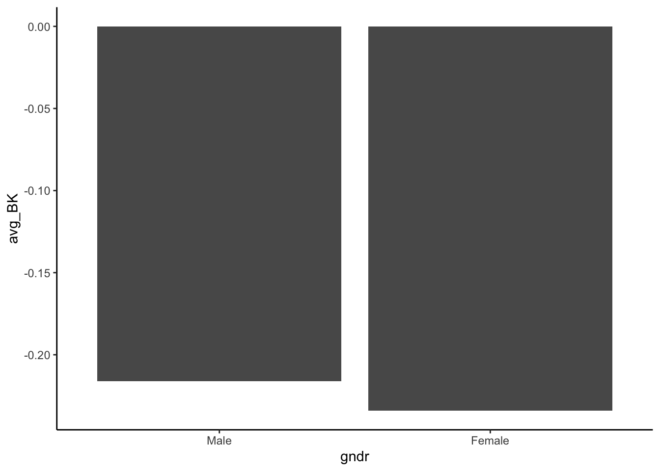
For example, let’s see if men or women are on average more exposed to globalization:

ess7 %>% 
  group_by(gndr) %>% 
  summarise(avg_BK = mean(BK, na.rm = T)) %>% 
  drop_na() %>%
  ggplot(aes(x = gndr, y = avg_BK)) +
    geom_col()

There is only a tiny difference: Women are very slightly less exposed to globalization than men.

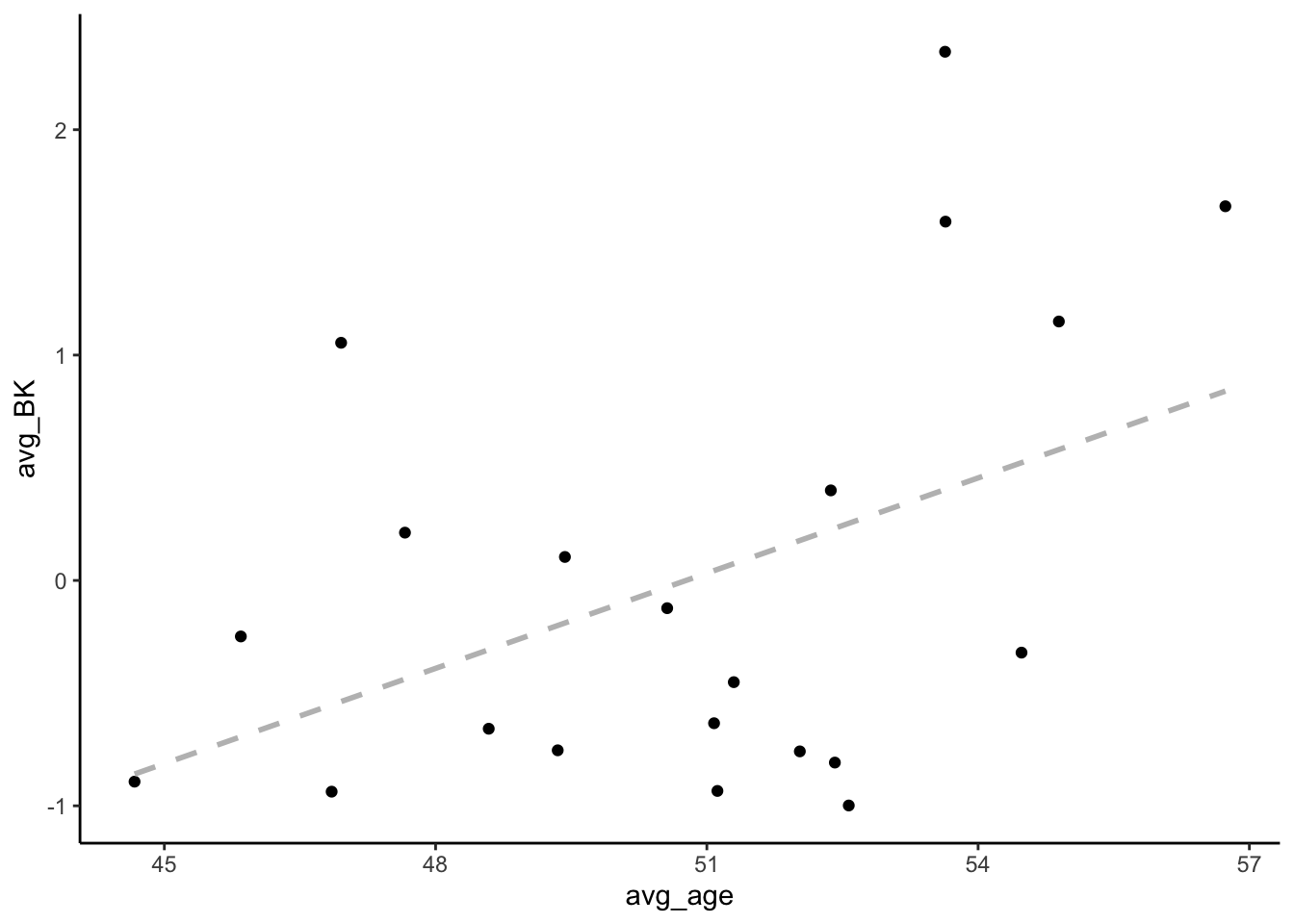
Next, we can see if there is a relation to age. To do that, we can calculate the average age in a given occupation and relate that average age to the vulnerability score in a scatterplot:

ess7 %>% 
  group_by(isco88_2d) %>% 
  summarise(avg_age = mean(agea, na.rm = T),
            avg_BK = mean(BK, na.rm = T)) %>% 
  drop_na() %>% 
  ggplot(aes(x = avg_age, y = avg_BK)) +
    geom_point() +
    geom_smooth(method = "lm", color = "grey", linetype = "dashed", se = F)
`geom_smooth()` using formula = 'y ~ x'

There does seem to be a positive relationship: Occupations where workers are older are also more exposed to globalization.

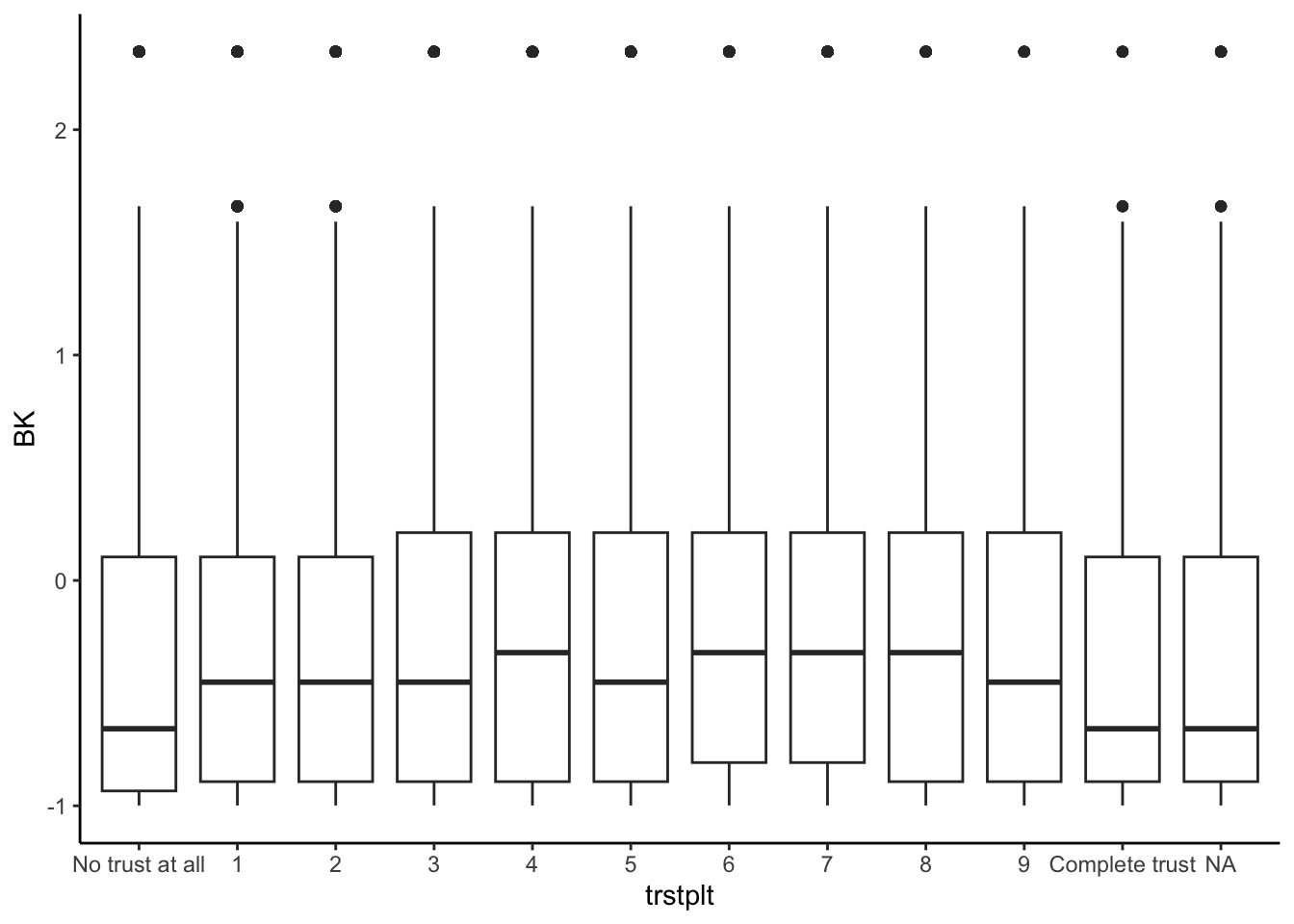
Finally, let’s see if exposure to globalization has political effects by testing if there is a relationship to trust in politicians. We do this with a box plot:

ess7 %>% 
  ggplot(aes(x = trstplt, y = BK)) +
    geom_boxplot()
Warning: Removed 8011 rows containing non-finite outside the scale range
(`stat_boxplot()`).

At least based on this (admittedly) very quick and superficial look at the data, there does not seem to be a strong relationship.

Next steps

Even if there is not link to political trust, maybe you can think of other variables that are measured in the ESS that globalization vulnerability could have an effect on? And maybe you can even think of macro-level variables that could make these effects stronger or weaker (and then use the other post to compare the effects of globalization vulnerability between two or more selected countries)?

Finally, you can also merge the vulnerability scores to other survey datasets such as the ISSP or the Eurobarometer so long as the survey dataset contains ISCO occupation scores.

References

Anelli, Massimo, Osea Giuntella, and Luca Stella. 2024. “Robots, Marriageable Men, Family, and Fertility.” Journal of Human Resources 59 (2): 443–69.
Autor, David H., David Dorn, and Gordon H Hanson. 2013. The China syndrome: Local labor market effects of import competition in the United States.” American Economic Review 103 (6): 2121–68.
Autor, David H., David Dorn, Gordon Hanson, and Kaveh Majlesi. 2020. “Importing Political Polarization? The Electoral Consequences of Rising Trade Exposure.” American Economic Review 110 (10): 3139–83.
Autor, David H., Frank Levy, and Richard J. Murnane. 2003. “The Skill Content of Recent Technological Change: An Empirical Exploration.” Quarterly Journal of Economics 118 (4): 1279–1333.
Blinder, Alan S, and Alan B Krueger. 2013. “Alternative Measures of Offshorability: A Survey Approach.” Journal of Labor Economics 31 (S1): S97–128.
Firpo, Sergio, Nicole M Fortin, and Thomas Lemieux. 2011. “Occupational Tasks and Changes in the Wage Structure.” IZA Discussion Paper 5542.
Goos, Maarten, Alan Manning, and Anna Salomons. 2014. “Explaining Job Polarization: Routine-Biased Technological Change and Offshoring.” American Economic Review 104 (8): 2509–26.
Heckscher, Eli F. 1919. “Utrikeshandelns Verkan på Inkomstfördelningen. Några Teoretiska Grundlinjer.” Ekonomisk Tidskrift 21: 1–31.
Ohlin, Bertil. 1933. Interregional and International Trade. Cambridge, MA: Harvard University Press.
Thewissen, Stefan, and David Rueda. 2019. “Automation and the Welfare State: Technological Change as a Determinant of Redistribution Preferences.” Comparative Political Studies 52 (2): 171–208.
Walter, Stefanie. 2010. “Globalization and the Welfare State: Testing the Microfoundations of the Compensation Hypothesis.” International Studies Quarterly 54 (2): 403–26.
Footnotes

  1. See https://ilostat.ilo.org/methods/concepts-and-definitions/classification-occupation/ for details on the ISCO classification.↩︎

  2. This works because the numbers reflect the hierarchical structure of the ISCO classification. If we cut off the last two numbers, we get to a higher level of aggregation. See https://ilostat.ilo.org/methods/concepts-and-definitions/classification-occupation/#elementor-toc__heading-anchor-2 for details.↩︎