  essround  idno cntry   gndr agea
1        7 12414    NO   Male   22
2        7  9438    NO Female   43
3        7 19782    NO Female   58
4        7 18876    NO Female   22
5        7 20508    NO   Male   84
6 7 19716 NO Male 621 + 1 = more
Being able to combine or merge different datasets is a critical skill for any (social, political, or economic) data analyst because, more often than not, the variables you need for your analysis are spread over different datasets. For example, many available datasets from peace & conflict research on fatalities related to wars and other types of conflict (as looked at in this post) contain just that – information about conflicts and their intensity. What they do not contain is variables that could potentially explain the incidence and intensity of conflicts, for example how democratic countries are (Maoz and Russett 1993; Oneal and Russett 1997) — which are available in other datasets (e.g., Lindberg et al. 2014; Boix et al. 2013). To be able to analyze these two variables, conflicts and democracy, and their relationships, you need to be able to merge the two datasets into one.
Fortunately, merging datasets is not as difficult as it might seem at first sight – functions like merge() from base R or left_join() and the other joining functions from dplyr() take care of most of the work (see also Urdinez and Cruz 2020, 11.2). You as the data analyst in charge really only need to take care of two things:
- You need to understand the structure of your datasets and which variable (or variables) uniquely identity each observation.
- You need to make sure that these identifying variables are exactly identical in each of the datasets you want to merge.
This may sound a bit cryptic to the uninitiated, but we will go through this step by step in the remainder of this post. More specifically, we will first go over some basics (dataset structures) and a common “snag” one encounters when working with macro- or country-level data: different country names and country codes. After that, we will do an example merging operation with two macro-level datasets, the dataset on conflict-related fatalities since 1989 from the Uppsala Conflict Data Program (as used here) and the Quality of Government Basic Dataset (Dahlberg et al. 2025).
I should also add that Steven V. Miller explains these things in two of his blog posts in probably a bit more detail:
- “A Quick Tutorial on Various State (Country) Classification Systems”
- “A Quick Tutorial on Merging Data with the *_join() Family of Functions in {dplyr}”
Do check them out! (I saw them too late, otherwise I wouldn’t have bothered writing my own, and clearly redundant, blog post…)
Dataset structures and identifying variables
Cross-sectional data
As you probably remember from your introductory data analysis or statistics course, datasets have different structures. Some are cross-sectional and contain data about a set of observations at one point in time. For example, data from the European Social Survey (ESS) contain information about a large number of survey respondents (observations) at a certain point in time – these data are cross-sectional survey data. This type of dataset will look more or less like this:
There are different respondents, and each of them is uniquely identified by their ID number (idno in this case). We also know that they come from Norway, were interviewed in round 7, and have different genders and ages.
Time series data
There are also datasets that follow a single observation over time – we call these time series data. An example is the airquality dataset that is one of the “built-in” datasets that come with R:
data(airquality)
head(airquality)
Ozone Solar.R Wind Temp Month Day
1 41 190 7.4 67 5 1
2 36 118 8.0 72 5 2
3 12 149 12.6 74 5 3
4 18 313 11.5 62 5 4
5 NA NA 14.3 56 5 5
6 28 NA 14.9 66 5 6If you look for the help file for this dataset with ?airquality, you will learn that it contains daily air quality measurements from New York between May and September 1973.
Note that the dataset contains two variables that relate to time: Month and Day. Obviously, each of these two variables by itself is useless. For example, just knowing that a measurement refers to day 2 is not helpful since the dataset covers four different months, each of which has a day 2. Therefore, to uniquely identify a given measurement or observation, we need both variables, Day and Month.
Time series cross-sectional data
There is also a third type of dataset that, simply put, follows a group of units over some period of time (as introduced here). This means this type of dataset combines time series and cross-sectional features, which is why we call this type of dataset a time series cross-sectional dataset (TSCS). Another commonly used term for this is panel data.1
Very commonly, TSCS data contain measurements of a set of countries over a number of years and will look more or less likely this:
# A tibble: 6 × 3
  cname  ccodealp  year
  <chr>  <chr>    <dbl>
1 Norway NOR       1994
2 Norway NOR       1995
3 Norway NOR       1996
4 Sweden SWE       1994
5 Sweden SWE       1995
6 Sweden SWE       1996
Each observation is a country-year (e.g., Norway in 1994, Norway in 1995, etc.) and we have those for multiple countries and multiple years.
Importantly, this means that each observation in such a dataset is uniquely identified by a combination of country and year. There are several observations from Norway and several from 1994, so neither the cname variable nor the year variable above uniquely identify each observation by itself – we always need both of them together to be able to tell what a given observation corresponds to.
We can always check if a variable or combination of variables uniquely identifies each observation in a dataset using the anyDuplicated() function from base R.2 If variables uniquely identify observations, there should be no duplicates – the function should return a 0.
For example, to check if the observations in the small dataset above (let’s assume it is called tscs) are uniquely identified by the cname variable, we run:
library(tidyverse)
tscs %>%
  {anyDuplicated(select(., cname)) == 0}
[1] FALSEThe result is obviously that cname does not uniquely identify each observation since each country is observed over different years. This means we also need the year variable to identify each observation:
tscs %>%
  {anyDuplicated(select(., cname,year)) == 0}
[1] TRUEOn country names and codes
The United Kingdom is officially also referred to as the “United Kingdom of Great Britain and Northern Ireland”, but sometimes simply as “Great Britain”. Similar, the United States are also called “USA” or “United States of America”, and the sample applies to a number of different countries (e.g., South Korea or the Netherlands). There are standardized codes that are supposed to fix this, one example being the ISO two- or three-digit country codes (where Norway would be NO or NOR) — but there are many different country coding conventions, and they can differ in some cases as well (the United States might be called US in one and USA in another).
This can be – and often is – a problem when we want to merge two TSCS datasets where countries are the units of observation. A common case is that one dataset contains two-digit ISO codes and the other contains their three-digit equivalents. In that case, Norway would be called NO in dataset 1 and NOR in dataset 2, and R will think these are two different units and will not be able to merge the observations.
Since this is such a common problem, Arel-Bundock, Enevoldsen, and Yetman (2018) put together the countrycode package that can convert different country names and codes back and forth, and which we can use to harmonize country variables across datasets. This is a very common operation we need to perform when merging two datasets.
The main function in countrycode is the countrycode() function, which has three main “arguments”:
countrycode::countrycode(sourcevar, origin, destination)It works, simply put, by taking a variable that identifies countries in a given dataset (sourcevar) and transforming it from its current encoding (origin) to a different one (destination).
For example, let’s say we want to convert the ccodealp variable in our little tscs practice dataset. As you can see below, the variable currently contains three-digit country codes for Norway and Sweden:
tscs# A tibble: 6 × 3
cname ccodealp year
<chr> <chr> <dbl>
1 Norway NOR 1994
2 Norway NOR 1995
3 Norway NOR 1996
4 Sweden SWE 1994
5 Sweden SWE 1995
6 Sweden SWE 1996Let’s say we need to convert this to its two-digit equivalent. To do this with countrycode, we need to specify ccodealp as the source variable, iso3c (“ISO three-character”) as the origin encoding, and iso2c as the destination encoding. We can use countrycode directly within mutate():
tscs %>%
  mutate(ccode_2d = countrycode::countrycode(sourcevar = ccodealp,
                                             origin = "iso3c",
                                             destination = "iso2c"))
# A tibble: 6 × 4
cname ccodealp year ccode_2d
<chr> <chr> <dbl> <chr>
1 Norway NOR 1994 NO
2 Norway NOR 1995 NO
3 Norway NOR 1996 NO
4 Sweden SWE 1994 SE
5 Sweden SWE 1995 SE
6 Sweden SWE 1996 SE In a real-world case, you first need to be sure what exactly the encoding of your country variable is — this information should be provided in the codebook for the dataset you are working with. You can then refer to the documentation for the countrycode package to see how you convert your existing variable into a the format you need.3
Example: Merging the Quality of Government and UCDP conflict fatality datasets
Let’s put all of this into action and merge two real-life research datasets, the Quality of Government (QoG) Standard Dataset (Teorell et al. 2025) and the Country-Year Dataset on Organized Violence within Country Borders from the Uppsala Conflict Data Program (UCDP) (Davies et al. 2025; Sundberg and Melander 2013).
Import
If you want to follow along, you can download them directly from https://www.gu.se/en/quality-government/qog-data/data-downloads/basic-dataset (important: we use the time series version of the QoG dataset, not the cross-sectional one, and we download it in Stata .dta format!) and https://ucdp.uu.se/downloads/index.html#orgviocy (here, we download it directly in the .RDS format that is native to R).
To import the datasets, we use read_dta() from haven and readRDS(), respectively:
ged <- readRDS("organizedviolencecy_v25_1.rds")
qog <- haven::read_dta("qog_bas_ts_jan25.dta")
Inspecting the data
As you can see from either the codebooks or the Environment tab, both datasets contain a number of different variables that measure countries and years. To keep things simple, we focus on the country_cy and year_cy variables in the UCDP dataset and the year and cname variables in the QoG dataset (wondering how to figure this out? This is why datasets have codebooks!).
Are observations uniquely identified?
Let’s first check that these variables really uniquely identify each observation:
qog %>%
  {anyDuplicated(select(., cname,year)) == 0}
[1] FALSEged %>%
{anyDuplicated(select(., country_cy,year_cy)) == 0}[1] TRUEThe UCDP dataset looks “clean”, but the QoG dataset has some repeated country-year pairs. This is how we can identify these “offending” countries:
qog %>%
  filter(duplicated(.[,c("cname","year")])) -> duplicates

unique(duplicates$cname)
[1] "Chile"
[2] "Congo (the Democratic Republic of the)"
[3] "Indonesia"
[4] "Syrian Arab Republic (the)" rm(duplicates)A closer inspection (the codebook is unfortunately quiet about this) that this is because one variable, ccodecow (more on that one comes below), is missing for half of these observations:
qog %>%
  filter(cname=="Chile") %>%
  head()
# A tibble: 6 × 279
cname_qog cname year ccodecow ccodealp ccodealp_year ccode_qog cname_year
<chr> <chr> <dbl> <dbl> <chr> <chr> <dbl> <chr>
1 Chile Chile 1946 155 CHL CHL46 152 Chile 1946
2 Chile Chile 1946 NA CHL CHL46 152 Chile 1946
3 Chile Chile 1947 155 CHL CHL47 152 Chile 1947
4 Chile Chile 1947 NA CHL CHL47 152 Chile 1947
5 Chile Chile 1948 155 CHL CHL48 152 Chile 1948
6 Chile Chile 1948 NA CHL CHL48 152 Chile 1948
# ℹ 271 more variables: ccode <dbl>, ajr_settmort <dbl>, atop_ally <dbl>,
# atop_number <dbl>, bci_bci <dbl>, bicc_gmi <dbl>, biu_offrel <dbl+lbl>,
# bl_asyf <dbl>, bl_asym <dbl>, bl_asymf <dbl>, bmr_dem <dbl>,
# bmr_demdur <dbl>, bti_aar <dbl>, bti_acp <dbl>, bti_cdi <dbl>,
# bti_ci <dbl>, bti_cps <dbl>, bti_cr <dbl>, bti_ds <dbl>, bti_eo <dbl>,
# bti_eos <dbl>, bti_ep <dbl>, bti_ffe <dbl>, bti_foe <dbl>, bti_ij <dbl>,
# bti_mes <dbl>, bti_muf <dbl>, bti_pdi <dbl>, bti_pp <dbl>, bti_prp <dbl>, …qog %>%
filter(cname=="Syrian Arab Republic (the)") %>%
head()# A tibble: 6 × 279
cname_qog cname year ccodecow ccodealp ccodealp_year ccode_qog cname_year
<chr> <chr> <dbl> <dbl> <chr> <chr> <dbl> <chr>
1 Syria Syrian A… 1946 652 SYR SYR46 760 Syria 1946
2 Syria Syrian A… 1946 652 SYR SYR46 760 Syria 1946
3 Syria Syrian A… 1946 NA SYR SYR46 760 Syria 1946
4 Syria Syrian A… 1946 NA SYR SYR46 760 Syria 1946
5 Syria Syrian A… 1947 652 SYR SYR47 760 Syria 1947
6 Syria Syrian A… 1947 652 SYR SYR47 760 Syria 1947
# ℹ 271 more variables: ccode <dbl>, ajr_settmort <dbl>, atop_ally <dbl>,
# atop_number <dbl>, bci_bci <dbl>, bicc_gmi <dbl>, biu_offrel <dbl+lbl>,
# bl_asyf <dbl>, bl_asym <dbl>, bl_asymf <dbl>, bmr_dem <dbl>,
# bmr_demdur <dbl>, bti_aar <dbl>, bti_acp <dbl>, bti_cdi <dbl>,
# bti_ci <dbl>, bti_cps <dbl>, bti_cr <dbl>, bti_ds <dbl>, bti_eo <dbl>,
# bti_eos <dbl>, bti_ep <dbl>, bti_ffe <dbl>, bti_foe <dbl>, bti_ij <dbl>,
# bti_mes <dbl>, bti_muf <dbl>, bti_pdi <dbl>, bti_pp <dbl>, bti_prp <dbl>, …qog %>%
filter(cname=="Indonesia") %>%
head()# A tibble: 6 × 279
cname_qog cname year ccodecow ccodealp ccodealp_year ccode_qog cname_year
<chr> <chr> <dbl> <dbl> <chr> <chr> <dbl> <chr>
1 Indonesia Indonesia 1950 850 IDN IDN50 360 Indonesia…
2 Indonesia Indonesia 1950 NA IDN IDN50 360 Indonesia…
3 Indonesia Indonesia 1951 850 IDN IDN51 360 Indonesia…
4 Indonesia Indonesia 1951 NA IDN IDN51 360 Indonesia…
5 Indonesia Indonesia 1952 850 IDN IDN52 360 Indonesia…
6 Indonesia Indonesia 1952 NA IDN IDN52 360 Indonesia…
# ℹ 271 more variables: ccode <dbl>, ajr_settmort <dbl>, atop_ally <dbl>,
# atop_number <dbl>, bci_bci <dbl>, bicc_gmi <dbl>, biu_offrel <dbl+lbl>,
# bl_asyf <dbl>, bl_asym <dbl>, bl_asymf <dbl>, bmr_dem <dbl>,
# bmr_demdur <dbl>, bti_aar <dbl>, bti_acp <dbl>, bti_cdi <dbl>,
# bti_ci <dbl>, bti_cps <dbl>, bti_cr <dbl>, bti_ds <dbl>, bti_eo <dbl>,
# bti_eos <dbl>, bti_ep <dbl>, bti_ffe <dbl>, bti_foe <dbl>, bti_ij <dbl>,
# bti_mes <dbl>, bti_muf <dbl>, bti_pdi <dbl>, bti_pp <dbl>, bti_prp <dbl>, …To keep things simple, we drop those countries:
qog %>%
  filter(!(cname %in% c("Chile","Indonesia",
                                        "Syrian Arab Republic (the)",
                                        "Congo (the Democratic Republic of the)"))) -> qog
Now the cname and year variables should uniquely identify each observation:
qog %>%
  {anyDuplicated(select(., cname,year)) == 0}
[1] TRUEWhich countries and years are covered?
Let’s now check which time periods the two datasets cover. Starting with the conflict dataset, we get:
min(ged$year_cy)[1] 1989max(ged$year_cy)[1] 2024In the case of the QoG data, we get:
min(qog$year)[1] 1946max(qog$year)[1] 2024Both datasets end in 2024, but the UCPD conflict dataset covers only the period after the fall of the Berlin Wall while the QoG dataset goes back to the year after World War II.
To make the datasets more compatible, we can now drop the years prior to 1989 from the QoG dataset:
qog %>%
  filter(year>=1989) -> qog
We can now, theoretically, check which countries are covered by each dataset with unique(), but this results in long lists of countries. To make this easier, we can start by looking at the number of countries in each dataset:
length(unique(ged$country_cy))[1] 199length(unique(qog$cname))[1] 197The UCPD dataset covers two more countries than the QoG dataset.
We can also see more in detail which countries (or, perhaps, country names) are included only in one but not in both datasets. To do that, we can use the setdiff() function from base R, which shows for any two vectors the items that are contained in one but not the other.
Important: We need to use this twice so we see which countries are covered in the UCDP dataset but not the QoG data, and vice versa. We start with the countries in the UCDP data that are not also in the QoG dataset:
setdiff(ged$country_cy,qog$cname) [1] "Antigua & Barbuda" "Bahamas"
[3] "Bolivia" "Bosnia-Herzegovina"
[5] "Brunei" "Cambodia (Kampuchea)"
[7] "Cape Verde" "Central African Republic"
[9] "Chile" "Comoros"
[11] "Congo" "Czech Republic"
[13] "DR Congo (Zaire)" "Dominican Republic"
[15] "East Timor" "Federated States of Micronesia"
[17] "Gambia" "Indonesia"
[19] "Iran" "Ivory Coast"
[21] "Kingdom of eSwatini (Swaziland)" "Kosovo"
[23] "Laos" "Madagascar (Malagasy)"
[25] "Moldova" "Myanmar (Burma)"
[27] "Netherlands" "Niger"
[29] "North Korea" "Philippines"
[31] "Russia (Soviet Union)" "Samoa (Western Samoa)"
[33] "Serbia (Yugoslavia)" "South Korea"
[35] "Syria" "Taiwan"
[37] "Tanzania" "United Arab Emirates"
[39] "United Kingdom" "United States of America"
[41] "Vatican City State" "Venezuela"
[43] "Vietnam (North Vietnam)" "Yemen (North Yemen)"
[45] "Yemen (South Yemen)" "Zimbabwe (Rhodesia)" This includes, as could be expected, some of the “usual suspects”: The UK, the US, the Netherlands, or the Koreas, which often have different names in different datasets.
Next, we check which countries are covered in the QoG but not the UCDP data:
setdiff(qog$cname,ged$country_cy) [1] "Antigua and Barbuda"
[2] "Bahamas (the)"
[3] "Bolivia (Plurinational State of)"
[4] "Bosnia and Herzegovina"
[5] "Brunei Darussalam"
[6] "Myanmar"
[7] "Cambodia"
[8] "Cabo Verde"
[9] "Central African Republic (the)"
[10] "Taiwan (Province of China)"
[11] "Comoros (the)"
[12] "Congo (the)"
[13] "Czechia"
[14] "Dominican Republic (the)"
[15] "Gambia (the)"
[16] "Iran (Islamic Republic of)"
[17] "Côte d'Ivoire"
[18] "Korea (the Democratic People's Republic of)"
[19] "Korea (the Republic of)"
[20] "Lao People's Democratic Republic (the)"
[21] "Madagascar"
[22] "Moldova (the Republic of)"
[23] "Netherlands (the)"
[24] "Niger (the)"
[25] "Micronesia (Federated States of)"
[26] "Philippines (the)"
[27] "Timor-Leste"
[28] "Russian Federation (the)"
[29] "Serbia"
[30] "Viet Nam"
[31] "Zimbabwe"
[32] "Yemen Democratic"
[33] "Sudan (the)"
[34] "Eswatini"
[35] "United Arab Emirates (the)"
[36] "USSR"
[37] "United Kingdom of Great Britain and Northern Ireland (the)"
[38] "Tanzania, the United Republic of"
[39] "United States of America (the)"
[40] "Venezuela (Bolivarian Republic of)"
[41] "Samoa"
[42] "Yemen"
[43] "Yugoslavia"
[44] "Serbia and Montenegro" This is about the same number, and again the “usual suspects”. Notice, for example, that Vietnam is spelled “Viet Nam” in the UCPD dataset.
As shown in the earlier post, there are three countries that are covered for only very brief periods in the UCDP dataset: The German Democratic Republic (“East Germany”), South Yemen, and Czechoslovakia. An easy solution is – again – to simply drop these countries:
ged %>%
  filter(!(country_cy %in% c("German Democratic Republic","Yemen (South Yemen)","Czechoslovakia"))) -> ged
Harmonizing the country variables
So far, we already had weed out some duplicate observations and found that, unsurprisingly, the country names differ between the two datasets. As explained earlier, we need to harmonize the country variables for the merge to work.
There are now different ways to handle this. We could either try to convert the country names in the cname variable in the QoG dataset to the format used in the country_cy variable in the UCDP dataset or vice versa. We could also try to convert both to ISO country codes and use these to merge the datasets.
A third option is to use the ccodecow variable that is contained in the QoG dataset (the one that caused problems earlier). This variable contains standardized country codes (in the form of numbers) from the Correlates of War project (COW; see https://correlatesofwar.org/). The advantage with using this variable is that it is already contained in one of the datasets, the QoG data. More importantly, the countrycode package “speaks” COW codes, so we can use the countrycode() function to convert the country names in the UCDP dataset to COW codes – and then we have everything we need in place!
To create COW country codes in the UCDP dataset, we specify that we want countrycode() to create a new variable called ccodcow in the UCDP dataset, and to do this by transforming the English country names contained in the country_cy variable into COW numerical codes (cown):
ged$ccodecow <- countrycode::countrycode(ged$country_cy,
                         origin = "country.name.en",
                         destination = "cown")
We can take a quick look at the UCDP dataset to see how the new variable looks like:4
ged %>%
  relocate(country_cy,year_cy,ccodecow)
# A tibble: 6,928 × 75
country_cy year_cy ccodecow country_id_cy region_cy main_govt_name_cy
<chr> <dbl> <dbl> <dbl> <chr> <chr>
1 Afghanistan 1989 700 700 Asia Government of Afghanist…
2 Afghanistan 1990 700 700 Asia Government of Afghanist…
3 Afghanistan 1991 700 700 Asia Government of Afghanist…
4 Afghanistan 1992 700 700 Asia Government of Afghanist…
5 Afghanistan 1993 700 700 Asia Government of Afghanist…
6 Afghanistan 1994 700 700 Asia Government of Afghanist…
7 Afghanistan 1995 700 700 Asia Government of Afghanist…
8 Afghanistan 1996 700 700 Asia Government of Afghanist…
9 Afghanistan 1997 700 700 Asia Government of Afghanist…
10 Afghanistan 1998 700 700 Asia Government of Afghanist…
# ℹ 6,918 more rows
# ℹ 69 more variables: sb_exist_cy <dbl>, sb_dyad_count_cy <dbl>,
# sb_dyad_ids_cy <chr>, sb_dyad_names_cy <chr>, sb_deaths_parties_cy <dbl>,
# sb_deaths_civilians_cy <dbl>, sb_deaths_unknown_cy <dbl>,
# sb_total_deaths_best_cy <dbl>, sb_total_deaths_high_cy <dbl>,
# sb_total_deaths_low_cy <dbl>, sb_intrastate_exist_cy <dbl>,
# sb_intrastate_dyad_count_cy <dbl>, sb_intrastate_dyad_ids_cy <chr>, …Merging the datasets
Now, after a long litany of inspection, cleaning, and harmonization, we can finally merge the datasets – which is, as promised, a fairly quick and simple operation: We use the left_join() function from the dplyr package, which takes one dataset and then merges it with all observations from another dataset that are contained in the first one based on the variables that uniquely identify the observations in each dataset.5
The code to do this looks as follows: We take the UCDP dataset and left_join() it with the QoG dataset along the ccodecow and year/year_cy variables and save the combined dataset as merged:
ged %>%
  left_join(qog, by = c("ccodecow" = "ccodecow",
                        "year_cy" = "year")) -> merged
The new merged dataset contains all variables that are contained in both datasets for all observations that in the UCDP dataset that are also present in the QoG dataset. We can see this more directly by looking at the number of variables (“columns”) per dataset:
ncol(ged)[1] 75ncol(qog)[1] 279ncol(merged)[1] 352The number of variables in merged is the number of variables in ged plus those in qog minus the two variables that were used to merge the dataset (ccodecow and year/year_cy).
Data exploration
Now that we have merged the datasets, we can do a bit of (quick and rough) data exploration to see if there is a relationship between how democratic a country is and how much conflict and violence happens in that country – we now have information on both aspects in one common dataset, so we can see if they are related!
To measure the incidence of conflict, we use the sb_total_deaths_best_cy variable from the UCDP dataset, which gives the best estimate of the number of fatalities due to state-based violence within the borders of a given country and in a given year (please see the codebook for details).
To measure democratic-ness, we use to different variables from the QoG dataset:
bmr_dem: A binary measure of democray (democratic in a given year, yes or no) from Boix, Miller, and Rosato (2013)vdem_libdem: A continuous measure of liberal democracy (to what degree is a country a liberal democracy in a given year?) that comes originally from the V-DEM dataset (Lindberg et al. 2014).
First, we see if there is a difference in the average number of conflict fatalities per year in democracies and non-democracies based on the binary measure of democracy (bmr_dem) and visualize the result in a bar graph:
merged %>%
  group_by(bmr_dem) %>%
  summarise(sumdeaths = sum(sb_total_deaths_best_cy, na.rm = T)) %>%
  drop_na(bmr_dem) %>%
  ggplot(aes(x = factor(bmr_dem), y = sumdeaths)) +
    geom_col() +
    scale_y_continuous(labels = scales::label_number()) +
    scale_x_discrete(labels = c("0" = "No", "1" = "Yes")) +
    labs( x = "Democracy (Boix/Miller/Rosato)",
          y = "Avg. conflict fatalities/year")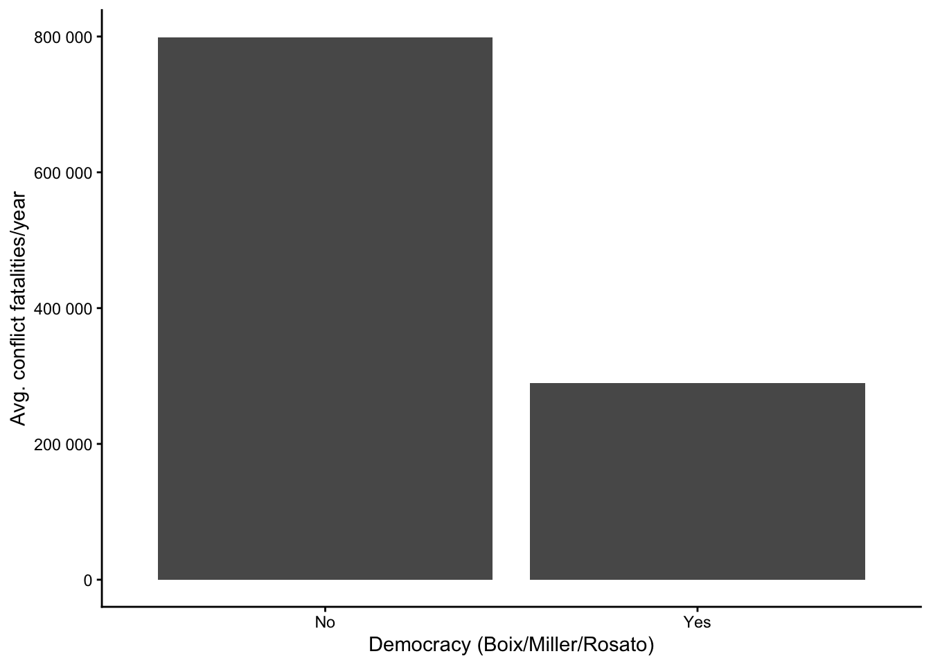
There clearly is a difference: Non-democracies (bmr_dem = 0) had on average around 800’000 fatalities per year, while the figure for democracies is slightly less than half of this. Obviously, one should not forget that conflict is overall relatively rare (see also https://cknotz.github.io/getstuffdone_blog/posts/conflict/#conflict-fatalities-across-countries), so these high averages are strongly driven by a few extreme cases with many fatalities. In other words, no, we obviously do not believe that Norway or Sweden had about 200’000 conflict deaths per year since 1989.
We might get a clearer picture by using the continuous measure of how liberal democratic a country is. Here, we group the data by country (using the ccodealp variable), calculate the average level of democratic-ness and the average number of conflict fatalities per country over the entire period of observation, and visualize the result in a scatter plot:
merged %>%
  group_by(ccodealp) %>%
  summarise(sumdeaths = sum(sb_total_deaths_best_cy, na.rm = T),
            avg_demo = mean(vdem_libdem, na.rm = T)) %>%
  filter(sumdeaths>1000) %>%
  ggplot(aes(x = avg_demo, y = sumdeaths)) +
    geom_text(aes(label = ccodealp)) +
    geom_smooth(method = "lm", se = F) +
    scale_y_continuous(labels = scales::label_number())
`geom_smooth()` using formula = 'y ~ x'Warning: Removed 3 rows containing non-finite outside the scale range
(`stat_smooth()`).Warning: Removed 3 rows containing missing values or values outside the scale range
(`geom_text()`).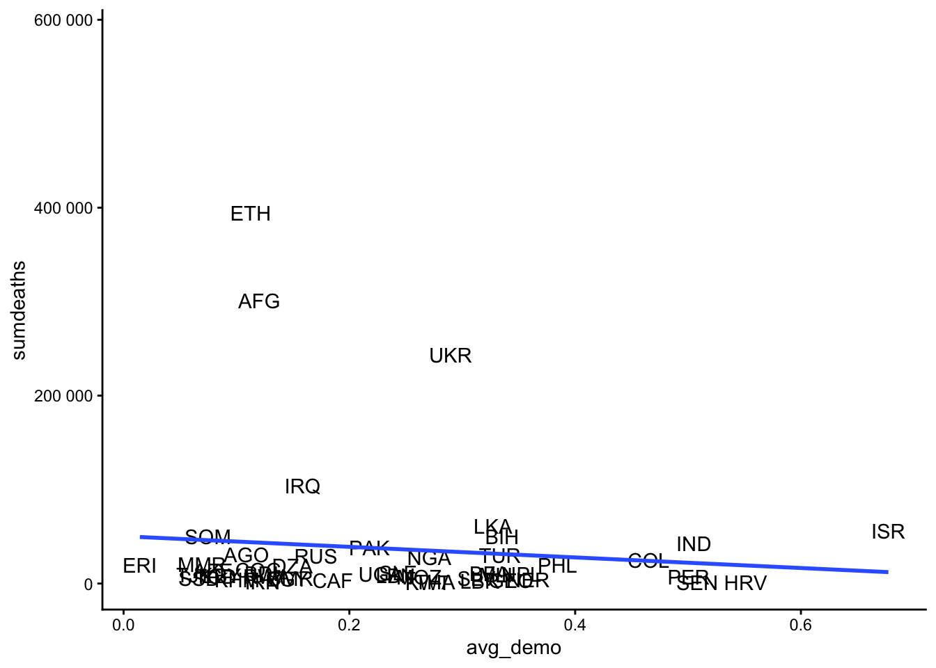
We find again a negative relationship – being more democratic is associated with fewer conflict fatalities – but this is to a large extent driven by a few countries with very violent state-based conflicts: Ethiopia, Afghanistan, Ukraine, and (although to a lesser extent) Iraq.
Conclusion
Being able to merge two (or more) datasets is a powerful skill because it allows you to analyze relationships between variables that are contained in two separate datasets.
After having gone through this post, you should see that the actual merging – using left_join() – is quite straightforward. You just need two datasets with overlapping observations and merge them along the variable (or variables) that uniquely identify each observation in each dataset.
The trickier thing is making sure that the datasets really are in a shape that they can be merged – that there are overlapping variables, which do identify each observation. There is no one standard solution here since each dataset is different. Solving this requires you to have a quite intimate knowledge of each of the datasets and to be able to convert variables, where necessary. For the former, being able to do data exploration in R is essential, as is reading (and understanding) the datasets’ codebooks. For the latter, countrycode is very helpful.
References
Arel-Bundock, Vincent, Nils Enevoldsen, and CJ Yetman. 2018. “countrycode: An R package to convert country names and country codes.” Journal of Open Source Software 3 (28): 848.
Beck, Nathaniel. 2001. “Time-Series-Cross-Section Data: What Have We Learned in the Past Few Years?” Annual Review of Political Science 4: 271–93.
Boix, Carles, Michael Miller, and Sebastian Rosato. 2013. “A Complete Data Set of Political Regimes, 1800–2007.” Comparative Political Studies 46 (12): 1523–54.
Dahlberg, Stefan, Aksel Sundström, Sören Holmberg, et al. 2025. The Quality of Government Basic Dataset, Version Jan25. The Quality of Government Institute, University of Gothenburg.
Davies, Shawn, Therése Pettersson, Margareta Sollenberg, and Magnus Öberg. 2025. “Organized Violence 1989–2024, and the Challenges of Identifying Civilian Victims.” Journal of Peace Research 62 (4).
Gleditsch, Kristian S, and Michael D Ward. 1999. “Interstate System Membership: A Revised List of the Independent States Since 1816.” International Interactions 25 (4): 393–413.
Lindberg, Staffan I, Michael Coppedge, John Gerring, and Jan Teorell. 2014. “V-Dem: A New Way to Measure Democracy.” Journal of Democracy 25 (3): 159–69.
Maoz, Zeev, and Bruce Russett. 1993. “Normative and Structural Causes of Democratic Peace, 1946–1986.” American Political Science Review 87 (3): 624–38.
Oneal, John R., and Bruce M. Russett. 1997. “The Classical Liberals Were Right: Democracy, Interdependence, and Conflict, 1950-1985.” International Studies Quarterly 41 (2): 267–94.
Sundberg, Ralph, and Erik Melander. 2013. “Introducing the UCDP Georeferenced Event Dataset.” Journal of Peace Research 50 (4): 523–32.
Teorell, Jan, Aksel Sundström, Sören Holmberg, et al. 2025. The Quality of Government Standard Dataset, v. Jan25. The Quality of Government Institute, University of Gothenburg.
Urdinez, Francisco, and Andres Cruz. 2020. R for Political Data Science: A Practical Guide. CRC Press.
Footnotes
While many use both terms interchangeably, it is more common to use the term panel when the dataset contains many observations but relatively few time points. The German Socio-Economic Panel (SOEP), for example, contains data for a large respondent sample (ca. 30.000 respondents per year) for up to 40 years. Here, the cross-sectional dimension is clearly dominant in terms of numbers. The term time series cross-sectional data is more often used for datasets that contain relatively few cross-sectional units – for example 20 to 50 countries – but over long periods of time. The V-Dem dataset (Lindberg et al. 2014) would be an example here. See also Beck (2001) for a more in-depth explanation.↩︎
See e.g., https://stackoverflow.com/a/65603253.↩︎
countrycodealso contains adata.framecalledcodelist_panelwith country and year information that takes into account that country names change over time (e.g., Germany was divided into East and West Germany before it reunified). Ideally, you use this dataset as a “link” when merging datasets that go far back in history (see also?countrycode::countrycode()).↩︎You may notice that the COW country codes overlap with the
country_id_cyvariable – but they are not exactly identical (see also the UCDP codebook and Gleditsch and Ward 1999).↩︎There are also other types of “mutating joins” in
dplyr; see https:dplyr.tidyverse.org/reference/mutate-joins.html for details.↩︎
Citation
BibTeX citation:
@online{knotz2025,
  author = {Knotz, Carlo},
  title = {Merging Macro-Level Data},
  date = {2025-10-10},
  url = {https://cknotz.github.io/getstuffdone_blog/posts/merging/},
  langid = {en}
}
For attribution, please cite this work as:
Knotz, Carlo. 2025. “Merging Macro-Level Data.” October 10.
https://cknotz.github.io/getstuffdone_blog/posts/merging/.