library(tidyverse)
theme_set(theme_classic())

cpds <- haven::read_dta("cpds_2024.dta")Macro-level questions and analyses (again)
This is another post on how to analyze country-level data, adding to the earlier post on how to do descriptive analyses (this one) and to the one on merging macro-level data (this one). What the earlier posts did not go into is how to do regression analyses with cross-country data, and this is what we are going to look into here.
Regression analyses with cross-country data work in principle the same way as regression analyses with other types of data – you specify a model that relates your dependent variable to one or more predictors and control variables, you estimate that model, and then you interpret the effects.
What makes macro-level analyses more complicated, however, is that macro-level data usually have a time dimension: They cover different countries over some period of time. This can range from a few decades like in the case of the Comparative Political Data Set (Armingeon et al. 2024) to multiple centuries like in the case of the V-Dem dataset (Lindberg et al. 2014). This is also why we call these types of datasets time series cross-sectional (TSCS) data: We have a cross-section of countries that are observed at multiple points in time.
Because TSCS data include observations of the same units (usually countries) over multiple points in time (usually years), they are sometimes also called “panel data”. However, this is a bit misleading, because panel data traditionally refer to panel survey data, which cover many respondents (typically 1000 or more) over a few time points (often 3-4). TSCS data, in contrast, usually cover only a moderate number of countries (20-35) over longer periods of time (see also Beck 2001).1
That being said, TSCS and panel data share the fact that they include a time dimension. This brings benefits (we can study changes over time and we simply have more observations to work with), but it also makes the dataset and therefore the analysis more complex. This complexity manifests itself in the fact that the results of analyses with TSCS data often change drastically after seemingly minor changes in model specifications (Wilson and Butler 2007) – and this is what can make these analyses so daunting to students.
However, TSCS (and panel) regression analyses do become easier and more predictable and stable if one understands a few core concepts:
- Cross-sectional and longitudinal variation
- Simpson’s Paradox
- Fixed- vs. random- vs. between-effects regression models
- Integration & cointegration (or, relatedly, unit roots and stationarity/non-stationarity)
The last ones, integration and co-integration, are concepts from time series analysis methods (see e.g., Box-Steffensmeier et al. 2014) and they refer, simply put, to how variables change over time: Some variables change smoothly over time and tend to return to a given stable equilibrium value, while others behave erratically and change in sudden (seemingly random) “fits and starts”. The former are considered “stationary”, the latter are considered to have “unit roots”. There is an older (and very short) article that illustrates the concept of unit roots, integration, and co-integration brilliantly with an analogy of a drunk and her dog (Murray 1994), and I would refer you to that one for further reading.2
The rest of this post will therefore go over the other three aspects with a focus on the main regression models for TSCS and the ideas behind them. You’ll also learn about panel-corrected standard errors (PCSEs), a key element in (political science) analyses of TSCS data Beck and Katz (1996). First, however, we will go over the structure of TSCS data and the types of variation they contain. We will use both artificial data and the Comparative Political Data Set (Armingeon et al. 2024) to illustrate the main points.
I should add that there are already other (excellent) introductory explanations of how to work with TSCS data in R by Urdinez & Cruz (2020, chap. 7) and Heiss (2020, chap. 13 & 14), but they lack (in my opinion) a user-friendly and easy conceptual introduction to the ideas behind the main regression models for TSCS and panel data. Working with these models and TSCS data becomes a lot easier once one understands these ideas (and the relatively simple math) behind these regression models.
Variation in TSCS data
Time series cross-sectional data contain observations of multiple units (usually countries) over some period of time (usually years). This means that this type of data can capture two basic forms of variation (see also Kellstedt and Whitten 2018, 2.3):
- Differences between units: Cross-sectional variation
- Changes over time: Longitudinal variation
To make this more concrete, we can look at some real-life examples from the Comparative Political Data Set [CPDS; Armingeon et al. (2024)] and use the simple data visualizations techniques that were covered in the earlier blog post.3
We will focus on two variables from the dataset for now:
structur, which measures the “rigidity” of countries’ political instititions, a.k.a., the number of “checks and balances” that make introducing reforms easier or more difficult (see also Huber et al. 1993; Immergut 1992; Immergut 1990; Tsebelis 2002)oldage_pmp, which measures the amount of government spending on old-age pensions in percent of countries’ gross domestic product (see also Adema and Ladaique 2009; Castles and Obinger 2007)
Cross-sectional variation
One way to look at cross-sectional variation is to look at countries’ average values on the two variables over the entire period of time for which we have observations.
cpds |>
  group_by(iso) |>
  summarise(avg_cons = mean(structur, na.rm = T)) |>
  ggplot(aes(x = avg_cons, y = reorder(iso, avg_cons))) +
    geom_linerange(aes(xmin = 0, xmax = avg_cons),
                 color = "grey") +
    geom_point() +
    labs(x = "Constitutional structure (avg.)",
         y = "")

cpds |>
  filter(year>=1980) |>
  group_by(iso) |>
  summarise(avg_pen = mean(oldage_pmp, na.rm = T)) |>
  ggplot(aes(x = avg_pen, y = reorder(iso, avg_pen))) +
    geom_linerange(aes(xmin = 0, xmax = avg_pen),
                   color = "grey") +
    geom_point() +
    labs(x = "Public pension spending (% GDP, avg.)",
         y = "")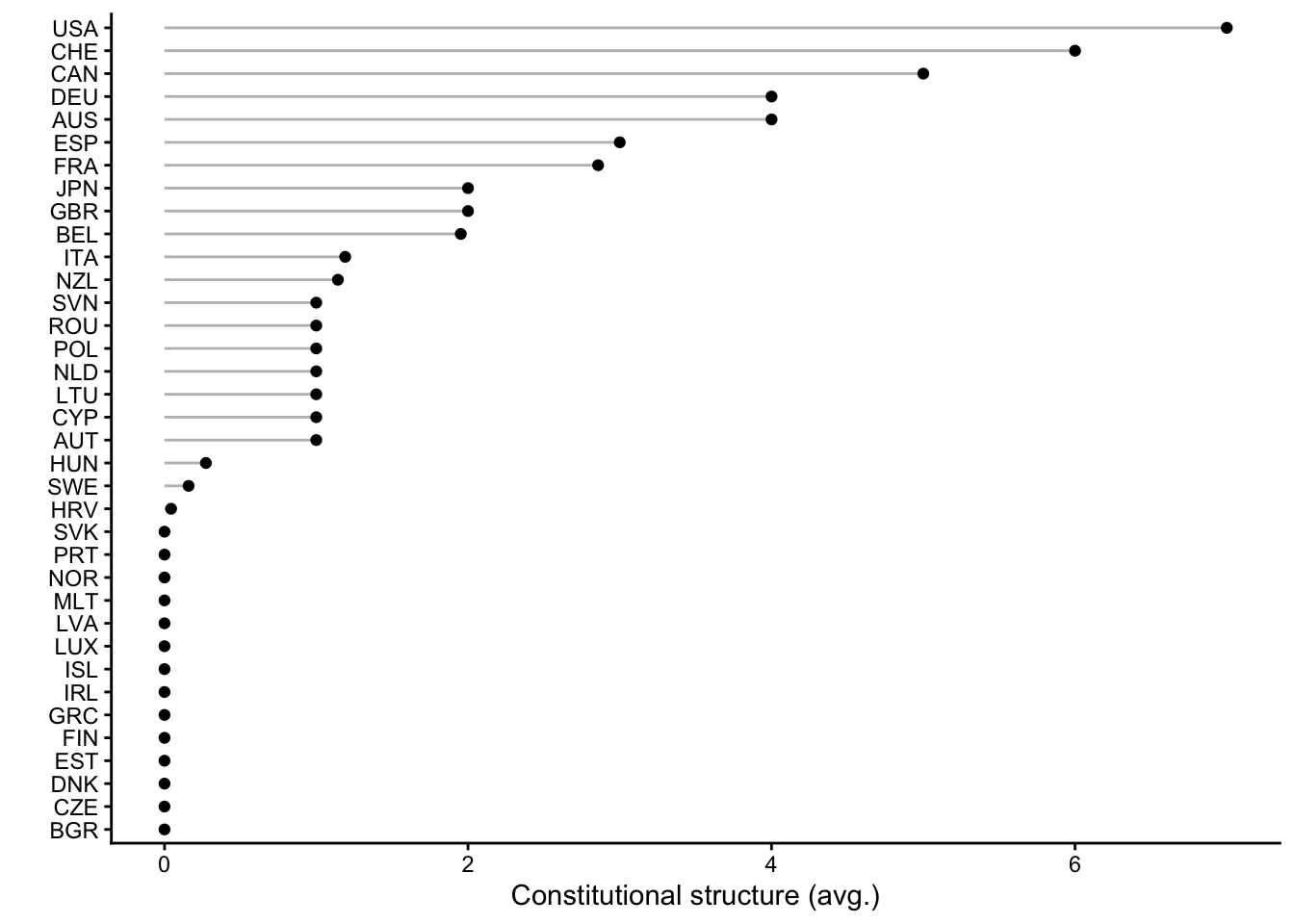
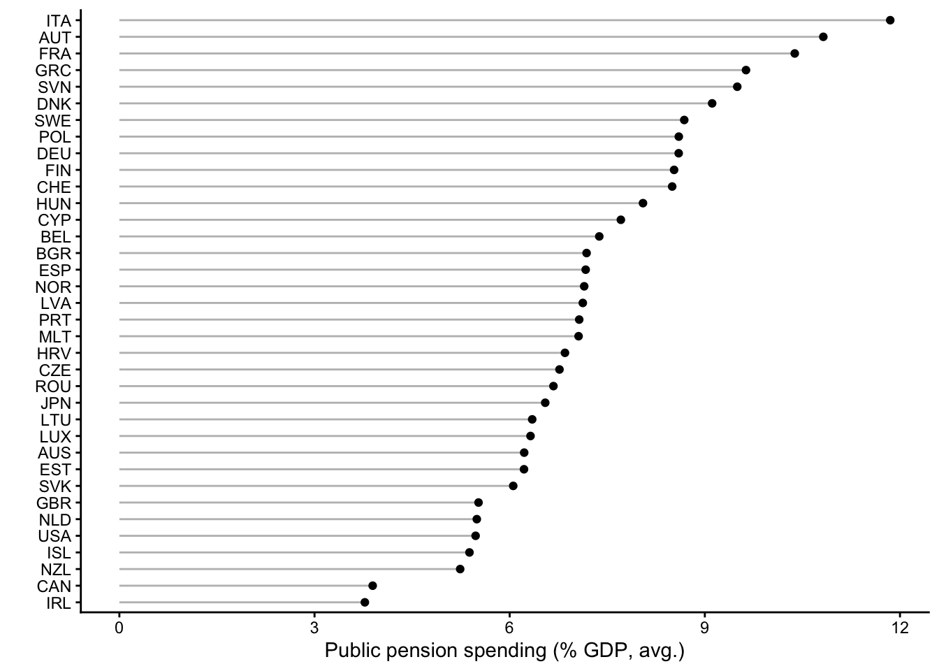
Figure 1 shows the results. On the left side, you see that countries differ in the “rigidity” of their political institutions. The United States and Switzerland stand out as countries with very rigid constitutions, where introducing reforms is very difficult, and this corresponds to what we know from more qualitative observations (Obinger 2002; Obama 2016). On the other end are a number of countries in different parts of Europe but also Israel, where there are few constraints. This does obviously not mean that these countries are dictatorships. It just means that there are few formal constraints on what a governing majority in parliament can do in day-to-day policymaking.
The other graph on the right shows that countries also differ quite a bit in how much they spend, on average, on old-age pensions. Conservative and southern European countries top the list, while more market-liberal countries like the United States, Canada, or Ireland are at the bottom.
Longitudinal variation
Obviously, by averaging the data by country, we brush away all the finer longitudinal changes over time within the different countries. To visualize this, we can use line graphs that are separated by country, as shown in Figure 2.
cpds |>
  drop_na(structur) |>
  ggplot(aes(x = year, y = structur)) +
    geom_line() +
    facet_wrap(~iso) +
    labs(x = "", y = "Constitutional structure")

cpds |>
  filter(year>=1980) |>
  ggplot(aes(x = year, y = oldage_pmp)) +
    geom_line() +
    facet_wrap(~iso) +
    labs(x = "", y = "Pension spending (%GDP)") +
    scale_x_continuous(breaks = seq(1980,2020,20))
Warning: Removed 2 rows containing missing values or values outside the scale range
(`geom_line()`).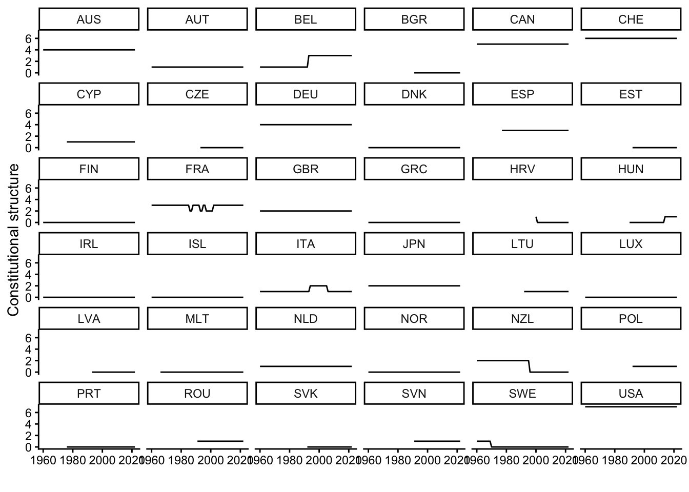
When you now look at the graph showing countries’ constitutional rigidity, you see that there are barely any changes over time. France is the big exception here since it introduced several constitutional changes over a decade or so, and there have also been changes in Belgium, Croatia, Hungary, Italy, New Zealand, and Sweden – but, overall, there is mainly stability.
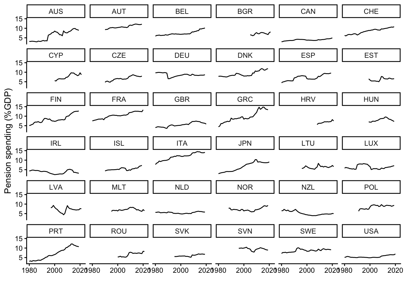
This contrasts with the pattern in the other graph that shows the development of public pension spending in each country. Many countries experienced significant increases over time (e.g., Greece, Portugal, Italy, Japan, Finland, France, or Switzerland), while spending stayed more constant in other countries (e.g., Poland, Germany, or the Netherlands). In all cases, however, there are small year-to-year changes, which is a clear difference to the completely flat lines in the graph above.
Simpson’s Paradox
The fact that TSCS data contain both cross-sectional and longitudinal variation makes regression analyses more challenging than when one uses a “simple” cross-sectional dataset like survey data from the European Social Survey.
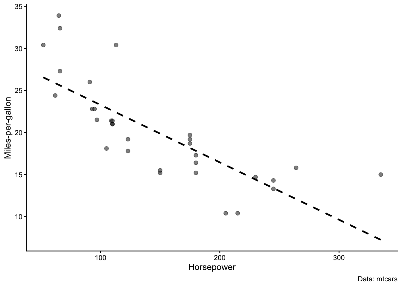
A normal regression model basically just draws a line through the data. The graph on the left in Figure 3 illustrates this with data from the mtcars dataset, where each observation is a car and cars differ in the strength of their engines (measured in horsepower) and in their fuel efficiency (measured in miles-per-gallon). Unsurprisingly, a more powerful engine with more horsepower means less fuel efficiency. In this case, the simple regression model works because the data are purely cross-sectional – there is no time-dimension or other complication.
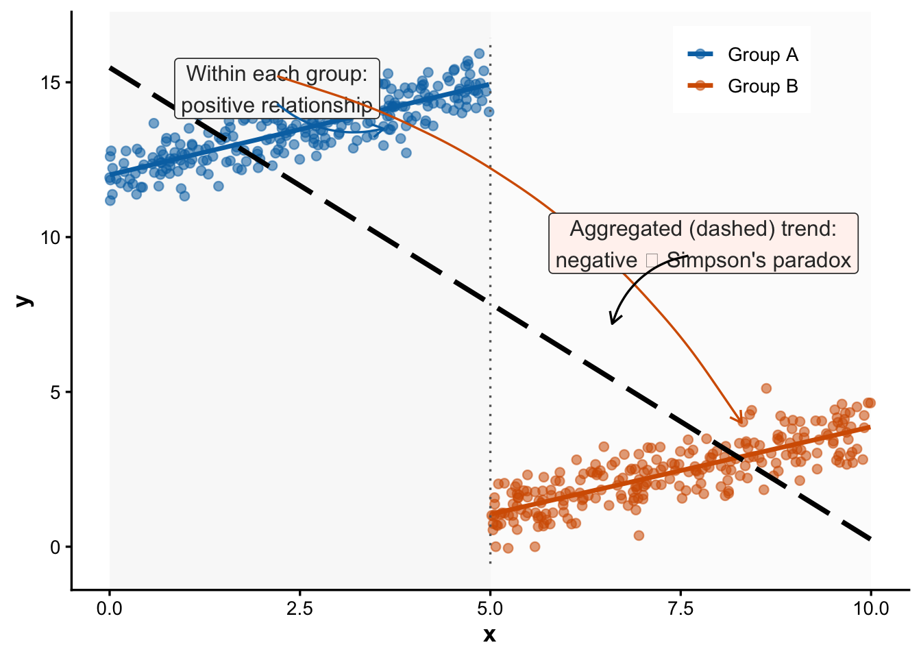
Now consider what can happen when we deal with a more complex dataset with two dimensions, which is shown in the graph on the right.4 A “naive” OLS regression (indicated with the thick black line) would find that there is a negative relationship between the two variables , x and y. However, within the two groups, the relationship is positive. This positive relationship is only correctly captured by a model that focuses exclusively on the variation within each group and ignores the differences between them (indicated by the two colored lines).
In principle, the “naive” OLS model is not really wrong – there is a negative relationship in the data as a whole. But the “naive” model is misleading, because it does not tell us the whole story. To get to that complete story, we need models that separate the between-group variation (the overall difference between groups A and B) from the within-group variation.
The following section introduces regression models that can achieve this.
Pooled, fixed-effects, and between-effects models
Statisticians have developed three basic regression model specifications for data that contain repeated observations of some group of units over time. Originally, they were developed for panel survey data, where researchers follow a larger (and often representative) sample of people over some period of time (often only a few weeks, months, or years) – i.e., data where we have many units but few time points. The models can in principle also be applied to TSCS data, where we usually have observations for many years but only a few countries – i.e., few units, but many time points (see also Beck 2001, 273).5
These models are available in R via the plm package (Croissant and Millo 2008), which you can install from CRAN with install.packages() and load with library(). In addition, we also use texreg (Leifeld 2013) to tabulate the results of the regression models:
# install.packages("plm")
library(plm)
library(texreg)
To illustrate how these models work, we will work with a tiny and artificial example dataset (pandat). This dataset contains only nine observations of three variables (x, y, c) for three groups (A, B, and C, measured with the u variable) at three points in time (1,2,3, measured with the t variable):
pandat# A tibble: 9 × 5
u t x c y
<chr> <dbl> <dbl> <dbl> <dbl>
1 A 1 1.4 2 0.6
2 A 2 1.7 2 -0.1
3 A 3 2.1 2 -0.2
4 B 1 2.1 1.5 4.6
5 B 2 2.5 1.5 4.3
6 B 3 2.7 1.5 3.8
7 C 1 1.9 3.5 2.4
8 C 2 2 3.5 2
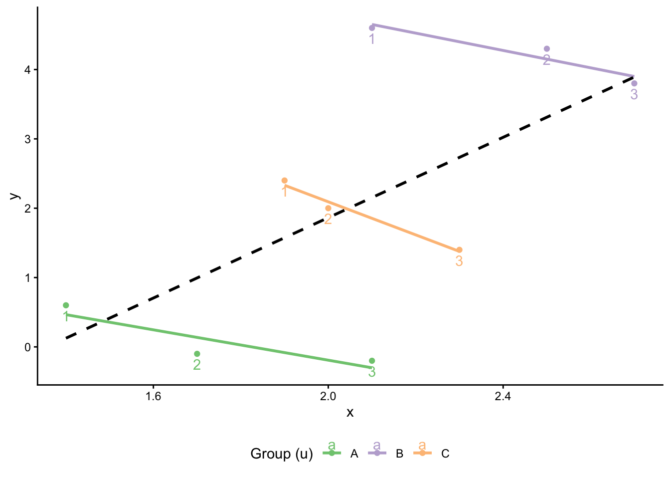
9 C 3 2.3 3.5 1.4When we visualize the patterns in the data (see Figure 4), we see that this is a textbook case of Simpson’s Paradox: Within each group, there is a negative relationship between x and y over time (time points are indicated as numbers). A naive OLS model, however, would find a positive relationship.
Naive or “pooled” regression
The first model specification is the “pooled” model. This model does what we did above: It pools all the different observations together and fits a line to the data. In other words, this model ignores the grouped structure of the data.
We can estimate this model with the plm() function from the plm package. This function works essentially like lm() or glm() with the exception that we also need to specify the structure of the data with the index argument (u designates the groups, t the time points) regardless of whether the model picks it up or not). We also need to specify the type of model we want to estimate (with the model argument):
pooled_plm <- plm::plm(y ~ x,
                index = c("u","t"),
                model = "pooling",
                data = pandat)
summary(pooled_plm)
Pooling Model
Call:
plm::plm(formula = y ~ x, data = pandat, model = "pooling", index = c("u",
"t"))
Balanced Panel: n = 3, T = 3, N = 9
Residuals:
Min. 1st Qu. Median 3rd Qu. Max.
-2.35327 -1.09434 0.13646 0.82619 2.44673
Coefficients:
Estimate Std. Error t-value Pr(>|t|)
(Intercept) -3.9312 2.8846 -1.3628 0.21515
x 2.8973 1.3664 2.1204 0.07167 .
---
Signif. codes: 0 '***' 0.001 '**' 0.01 '*' 0.05 '.' 0.1 ' ' 1
Total Sum of Squares: 26.949
Residual Sum of Squares: 16.409
R-Squared: 0.39111
Adj. R-Squared: 0.30412
F-statistic: 4.49627 on 1 and 7 DF, p-value: 0.071675As expected, the model naively pools the data and captures the positive overall relationship between x and y with a positive (and borderline significant) coefficient. It completely ignores the negative relationship between the groups.
For comparison, we can also estimate a standard OLS model with lm():
pooled_lm <- lm(y ~ x,
          data = pandat)
summary(pooled_lm)
Call:
lm(formula = y ~ x, data = pandat)

Residuals:
    Min      1Q  Median      3Q     Max
-2.3533 -1.0943  0.1365  0.8262  2.4467

Coefficients:
            Estimate Std. Error t value Pr(>|t|)
(Intercept)   -3.931      2.885  -1.363   0.2152
x              2.897      1.366   2.120   0.0717 .
---
Signif. codes:  0 '***' 0.001 '**' 0.01 '*' 0.05 '.' 0.1 ' ' 1

Residual standard error: 1.531 on 7 degrees of freedom
Multiple R-squared:  0.3911,    Adjusted R-squared:  0.3041
F-statistic: 4.496 on 1 and 7 DF,  p-value: 0.07167
The results are exactly identical. This is easier to see when we put the results side-by-side in a single table:
screenreg(list(pooled_plm,pooled_lm),
          stars = 0.05,
          custom.model.names = c("Pooling (plm)",
                                 "Regular OLS"))
=======================================
             Pooling (plm)  Regular OLS
---------------------------------------
(Intercept)  -3.93          -3.93
             (2.88)         (2.88)
x             2.90           2.90
             (1.37)         (1.37)
---------------------------------------
R^2           0.39           0.39
Adj. R^2      0.30           0.30
Num. obs.     9              9
=======================================
* p < 0.05
The between-effects model
As explained above, the problem with the pooled model is that naively throws together the cross-sectional and longitudinal variation in the data. We can get better answers by separating the two types of variation, and the first type of model that does this is the between-effects model. As the name suggests, the between-effects model focuses completely on the differences between the units and ignores all longitudinal variation over time.
The between-effects model is also almost embarrassingly simple: All we do is what we did in Figure 1 above: We calculate average values per unit, which means that we eliminate the time-dimension from the data. Then we use the resulting aggregated data in a regular OLS regression.
To show how this works, we do this first by hand and create an aggregated version of the pandat dataset:
pandat |>
  group_by(u) |>
  summarise(avg_y = mean(y),
            avg_x = mean(x)) -> pan_ag
This dataset contains only the positive cross-sectional or between-unit relationship in the data:
pan_ag |>
  ggplot(aes(x = avg_x, y = avg_y)) +
    geom_text(aes(label = u)) +
    geom_smooth(method = "lm", se = F)
`geom_smooth()` using formula = 'y ~ x'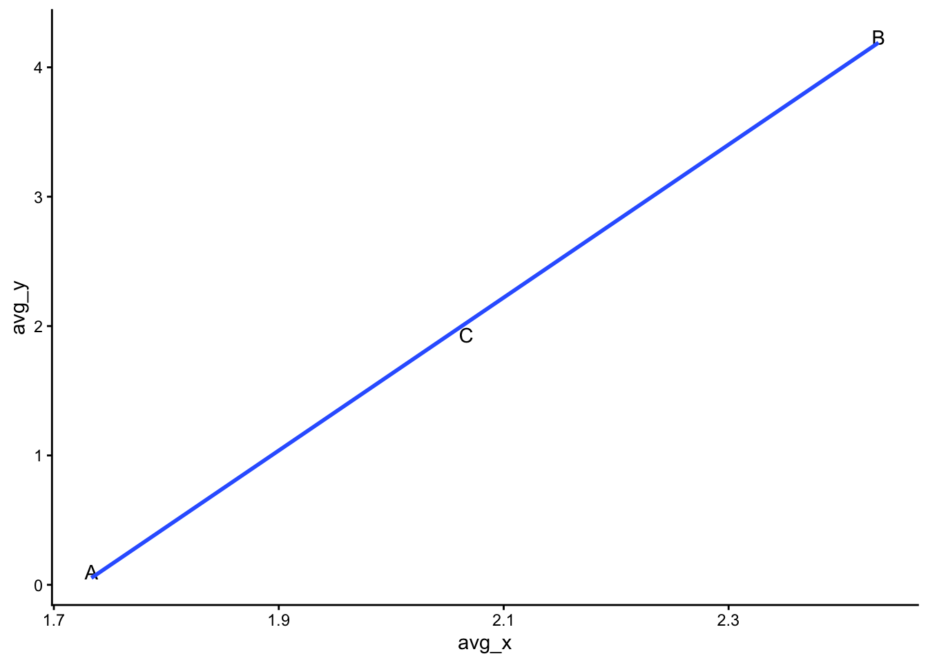
If we use this aggregated dataset in a conventional OLS regression, we find the expected positive (and now significant) relationship:
be_ols <- lm(avg_y ~ avg_x,
         data = pan_ag)
summary(be_ols)
Call:
lm(formula = avg_y ~ avg_x, data = pan_ag)

Residuals:
       1        2        3
 0.04708  0.04280 -0.08988

Coefficients:
            Estimate Std. Error t value Pr(>|t|)
(Intercept) -10.1926     0.4664  -21.85   0.0291 *
avg_x         5.9109     0.2224   26.58   0.0239 *
---
Signif. codes:  0 '***' 0.001 '**' 0.01 '*' 0.05 '.' 0.1 ' ' 1

Residual standard error: 0.1101 on 1 degrees of freedom
Multiple R-squared:  0.9986,    Adjusted R-squared:  0.9972
F-statistic: 706.4 on 1 and 1 DF,  p-value: 0.02394
Now compare this to the between model specification in plm():
be_plm <- plm::plm(y ~ x,
                index = c("u","t"),
                model = "between",
                data = pandat)
summary(be_plm)
Oneway (individual) effect Between Model
Call:
plm::plm(formula = y ~ x, data = pandat, model = "between", index = c("u",
"t"))
Balanced Panel: n = 3, T = 3, N = 9
Observations used in estimation: 3
Residuals:
A B C
0.047080 0.042800 -0.089879
Coefficients:
Estimate Std. Error t-value Pr(>|t|)
(Intercept) -10.19260 0.46644 -21.852 0.02911 *
x 5.91088 0.22239 26.578 0.02394 *
---
Signif. codes: 0 '***' 0.001 '**' 0.01 '*' 0.05 '.' 0.1 ' ' 1
Total Sum of Squares: 8.5785
Residual Sum of Squares: 0.012127
R-Squared: 0.99859
Adj. R-Squared: 0.99717
F-statistic: 706.416 on 1 and 1 DF, p-value: 0.023941The results are again exactly identical:
screenreg(list(be_ols,be_plm),
          stars = 0.05,
          custom.model.names = c("OLS with aggregated data",
                                 "Between-effects model (plm)"))
==================================================================
             OLS with aggregated data  Between-effects model (plm)
------------------------------------------------------------------
(Intercept)  -10.19 *                  -10.19 *
              (0.47)                    (0.47)
avg_x          5.91 *
              (0.22)
x                                        5.91 *
                                        (0.22)
------------------------------------------------------------------
R^2            1.00                      1.00
Adj. R^2       1.00                      1.00
Num. obs.      3                         3
==================================================================
* p < 0.05
The within- or fixed-effects model
As above, aggregating the data is inefficient because we lose all the longitudinal variation. Also, depending on the theory or hypothesis we want to test, we may need to focus on the within-group variation in our analysis. In those cases, the between-effects model (or the pooled model) will not get us very far.
If we want to focus on the within- or longitudinal variation, we can use the third alternative, which is the within-model. It is also known as the fixed-effects (FE) model. This model is, in principle, also very simple. One way to estimate this model is to simply add dummy variables for the different group units to the model (leaving one group out as the baseline). However, this adds extra variables to the model and therefore eats up statistical power that we often want to focus instead on the main effect of interest, here the relationship between x and y.
There is therefore another way to estimate this model, which is to de-mean the data and then estimate a linear regression on the resulting dataset. This means that we calculate average values for each of the variables in the model and then subtract the average from each observation. In a way, de-meaning the data is the opposite to calculating the group averages in the between-effects model.
This de-meaning of the data is a simple operation that we can again do by hand:
pandat |>
  group_by(u) |>
  mutate(avg_x = mean(x),
         avg_y = mean(y)) |>
  ungroup() |>
  mutate(diff_x = x - avg_x,
         diff_y = y - avg_y) -> pandat
Then we use the de-meaned data in a conventional OLS regression:
fe_ols <- lm(diff_y ~ diff_x,
          data = pandat)
summary(fe_ols)
Call:
lm(formula = diff_y ~ diff_x, data = pandat)

Residuals:
     Min       1Q   Median       3Q      Max
-0.24551 -0.08846 -0.02436  0.15769  0.23910

Coefficients:
              Estimate Std. Error t value Pr(>|t|)
(Intercept) -1.616e-16  6.222e-02   0.000  1.00000
diff_x      -1.365e+00  2.589e-01  -5.275  0.00115 **
---
Signif. codes:  0 '***' 0.001 '**' 0.01 '*' 0.05 '.' 0.1 ' ' 1

Residual standard error: 0.1867 on 7 degrees of freedom
Multiple R-squared:  0.799, Adjusted R-squared:  0.7703
F-statistic: 27.82 on 1 and 7 DF,  p-value: 0.001155
Notice that the coefficient on x now switches its sign: It is now negative – which means that the model now captures the negative relationship between x and y within each group.
When using the plm() function, we simply specify within as the model – but we use the original data. plm() takes care of the de-meaning for us:
fe_plm <- plm::plm(y ~ x,
                index = c("u","t"),
                model = "within",
                data = pandat)
summary(fe_plm)
Oneway (individual) effect Within Model
Call:
plm::plm(formula = y ~ x, data = pandat, model = "within", index = c("u",
"t"))
Balanced Panel: n = 3, T = 3, N = 9
Residuals:
1 2 3 4 5 6 7 8
0.044872 -0.245513 0.200641 -0.088462 0.157692 -0.069231 0.239103 -0.024359
9
-0.214744
Coefficients:
Estimate Std. Error t-value Pr(>|t|)
x -1.36538 0.30629 -4.4579 0.006654 **
---
Signif. codes: 0 '***' 0.001 '**' 0.01 '*' 0.05 '.' 0.1 ' ' 1
Total Sum of Squares: 1.2133
Residual Sum of Squares: 0.24391
R-Squared: 0.79898
Adj. R-Squared: 0.67836
F-statistic: 19.8725 on 1 and 5 DF, p-value: 0.0066536If you take a very careful look at the results, you see that the coefficient estimate (\(\beta\)) is exactly identical to the one we got in the OLS model on the de-meaned data. However, the standard error and t- and p-values are different!
The reason for this is that we use up some of the information in the data (i.e., degrees of freedom) when we calculate the group-averages in the first step. This information is then technically not available when when we calculate standard errors and p-values.6 The plm() function automatically makes this degree-of-freedom adjustment, but not the naive lm() function, hence the different results.
Now compare this to the “dummy” specification:
fe_dum <- lm(y ~ x + u,
          data = pandat)
summary(fe_dum)
Call:
lm(formula = y ~ x + u, data = pandat)

Residuals:
       1        2        3        4        5        6        7        8
 0.04487 -0.24551  0.20064 -0.08846  0.15769 -0.06923  0.23910 -0.02436
       9
-0.21474

Coefficients:
            Estimate Std. Error t value Pr(>|t|)
(Intercept)   2.4667     0.5460   4.518 0.006296 **
x            -1.3654     0.3063  -4.458 0.006654 **
uB            5.0891     0.2802  18.165 9.29e-06 ***
uC            2.2885     0.2072  11.043 0.000106 ***
---
Signif. codes:  0 '***' 0.001 '**' 0.01 '*' 0.05 '.' 0.1 ' ' 1

Residual standard error: 0.2209 on 5 degrees of freedom
Multiple R-squared:  0.9909,    Adjusted R-squared:  0.9855
F-statistic: 182.5 on 3 and 5 DF,  p-value: 1.583e-05
Now we have two additional variables in the model, the dummies for groups B and C (group A is omitted and measured with the intercept). If you take a careful look, you will notice that the estimate for the coefficient on x is now exactly identical to the estimate we got from the plm() function. This is because the dummy-specification explicitly adjusts for the degrees of freedom by adding additional coefficients to the model (which use up information in the estimation).
We can again put the results side-by-side to see more clearly where they differ:
screenreg(list(fe_ols,fe_plm,fe_dum),
          stars = 0.05,
          custom.model.names = c("Regular OLS (dem. data)",
                                 "Fixed-effects (plm)",
                                 "Fixed-effects (dummies)"))
==================================================================================
             Regular OLS (dem. data)  Fixed-effects (plm)  Fixed-effects (dummies)
----------------------------------------------------------------------------------
(Intercept)  -0.00                                          2.47 *
             (0.06)                                        (0.55)
diff_x       -1.37 *
             (0.26)
x                                     -1.37 *              -1.37 *
                                      (0.31)               (0.31)
uB                                                          5.09 *
                                                           (0.28)
uC                                                          2.29 *
                                                           (0.21)
----------------------------------------------------------------------------------
R^2           0.80                     0.80                 0.99
Adj. R^2      0.77                     0.68                 0.99
Num. obs.     9                        9                    9
==================================================================================
* p < 0.05
Again, the estimates of the coefficient on x are exactly identical across the three models, but the standard error is a bit lower in the first model than in the other two (which are exactly identical). You probably also notice that the within- or fixed-effects model estimated with plm() does not contain an intercept.
In any case, the fixed-effects or within-specification correctly captures the within-variation in the data, meaning the negative relationship between x and y within each group.
Fixed-effects with constant variables
You might now ask why we don’t just always use the fixed-effects (FE) model for anything? One of the problems with the FE model is that it cannot capture the effects of variables that are either constant over time or change only very rarely and slowly – the constitutional constraints variable is one of the textbook examples.
To see why, we can estimate a FE model with the one variable in our practice dataset that does not change over time (c, for “constant”):
pandat# A tibble: 9 × 9
u t x c y avg_x avg_y diff_x diff_y
<chr> <dbl> <dbl> <dbl> <dbl> <dbl> <dbl> <dbl> <dbl>
1 A 1 1.4 2 0.6 1.73 0.1 -0.333 0.5
2 A 2 1.7 2 -0.1 1.73 0.1 -0.0333 -0.2
3 A 3 2.1 2 -0.2 1.73 0.1 0.367 -0.3
4 B 1 2.1 1.5 4.6 2.43 4.23 -0.333 0.367
5 B 2 2.5 1.5 4.3 2.43 4.23 0.0667 0.0667
6 B 3 2.7 1.5 3.8 2.43 4.23 0.267 -0.433
7 C 1 1.9 3.5 2.4 2.07 1.93 -0.167 0.467
8 C 2 2 3.5 2 2.07 1.93 -0.0667 0.0667
9 C 3 2.3 3.5 1.4 2.07 1.93 0.233 -0.533 Notice what happens when we do the de-meaning operation with this variable:
pandat |>
  group_by(u) |>
  mutate(avg_c = mean(c)) |>
  ungroup() |>
  mutate(diff_c = c - avg_c) -> pandat

pandat |>
  select(u,t,c,avg_c,diff_c)
# A tibble: 9 × 5
u t c avg_c diff_c
<chr> <dbl> <dbl> <dbl> <dbl>
1 A 1 2 2 0
2 A 2 2 2 0
3 A 3 2 2 0
4 B 1 1.5 1.5 0
5 B 2 1.5 1.5 0
6 B 3 1.5 1.5 0
7 C 1 3.5 3.5 0
8 C 2 3.5 3.5 0
9 C 3 3.5 3.5 0The resulting variable, diff_c (which measures the deviations of each variable from the group-specific means) contains only zeros! This is only logical: The variable does not change over time, so each individual observation is exactly identical to the group-specific mean. When we then subtract the two, we get only zeros.
plm() will now simply refuse to estimate the model:
fe_plm_c <- plm(y ~ c,
                index = c("u","t"),
                model = "within",
                data = pandat)
Error in plm.fit(data, model, effect, random.method, random.models, random.dfcor, : empty modelsummary(fe_plm_c)Error: object 'fe_plm_c' not foundWhich model should I now choose?
The main difference between the three regression models we went over is which type of variation they focus on (i.e., how they “slice” the data):
- The “pooling” model simply pools all the data together and draws a best-fitting line through them. It does not differentiate between between-country and over-time variation and can therefore produce very misleading results (due to Simpson’s Paradox; see above).
- The “between-effects” model is simply a regression model that is fitted on country-by-country averages. This eliminates the time-dimension from the data and focuses the analysis exclusively on between-country differences (cross-sectional variation).
- The “fixed-effects” model focuses on deviations from the country-by-country averages, which means that it eliminates all cross-sectional variation from the data and focuses the analysis on the longitudinal or over-time variation in the data.
Because these models focus on different types of variation, you use them for different types of analyses. As always, which model you use depends on the theory or hypothesis you want to test.
First, you might be interested in stable differences between countries or in the effects of variables that rarely or never change over time. Political institutions are the textbook example for the latter (as shown above). They basically never change, which means they are a stable cross-sectional feature of different countries.7 In such cases, when you are interested in stable cross-sectional variation, you should use the between-effects model. For example, Iversen and Soskice (2006) used the between-effects regression model in their study of the effects of electoral systems on government redistribution.
A second scenario is that you are interested in longitudinal/over-time changes. For example, an older literature in political science and sociology was interested in how economic globalization (increases in international trade and financial transactions across countries) affects the welfare state (Cerny 1997; Sassen 1996; Iversen and Cusack 2000; Burgoon 2001; Garrett and Mitchell 2001; Brady et al. 2005). In that case, the fixed-effects model would be a natural choice because it focuses the analysis on over-time changes (how increased globalization leads to changes in welfare state institutions or outcomes) and removes the effects of stable country differences. You can estimate the fixed-effects model either by including dummy-variables for your countries (or other cross-sectional units) or with the “official” within estimator built into the plm package (as shown above.)
Third, there are some who still prefer the “pooling” model (e.g., Huber et al. 1993; Huber and Stephens 2000, 2001), and it can indeed be an appropriate model for some types of analyses. One case would be when you are doing analyses that look at between-country and longitudinal variation simultaneously (e.g., when you are interested in how patterns of change differ between countries). For example, you might be interested in how the effect of globalization on welfare states (longitudinal variation) depends on political institutions (cross-sectional variation).8 Still, you need to be cautious when you use the “pooling” model (see also Wilson and Butler 2007, 104–5).
Estimation issues & panel-corrected standard errors
OLS assumptions and why they will usually not hold in the case of TSCS data
You might remember that a standard linear regression (OLS) model is based on a few critical assumptions about the underlying data (see e.g., Kellstedt and Whitten 2018, 9.5). One of these assumptions is no autocorrelation: Two different observations in your dataset cannot be related to each other. In a survey dataset, where all observations are individual and randomly sampled people from different parts of a given country, this assumption is plausible: Respondent #1 is not directly connected to respondent #2, so the data from respondent #1 are not correlated with those from respondent number #2.
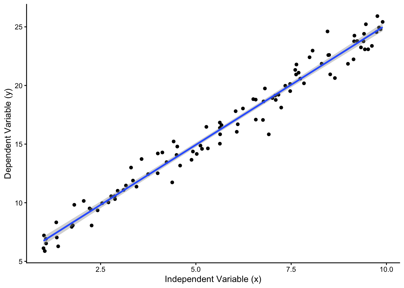
A second assumption is that of homoscedasticity, meaning that there cannot any form of pattern in the residuals (usually called \(\epsilon_i\)) from the regression model, i.e., the unexplained variation that the model does not pick up. No regression model will fit a given dataset perfectly, and there are always some observations that are well-explained by the model and that lie on or close to the regression line, and other observations that are “weird” and lie far away from the regression line. This is not a problem as long as there is no systematic pattern to these deviations from the regression line. The graph on the left in Figure 5 visualizes this ideal case.
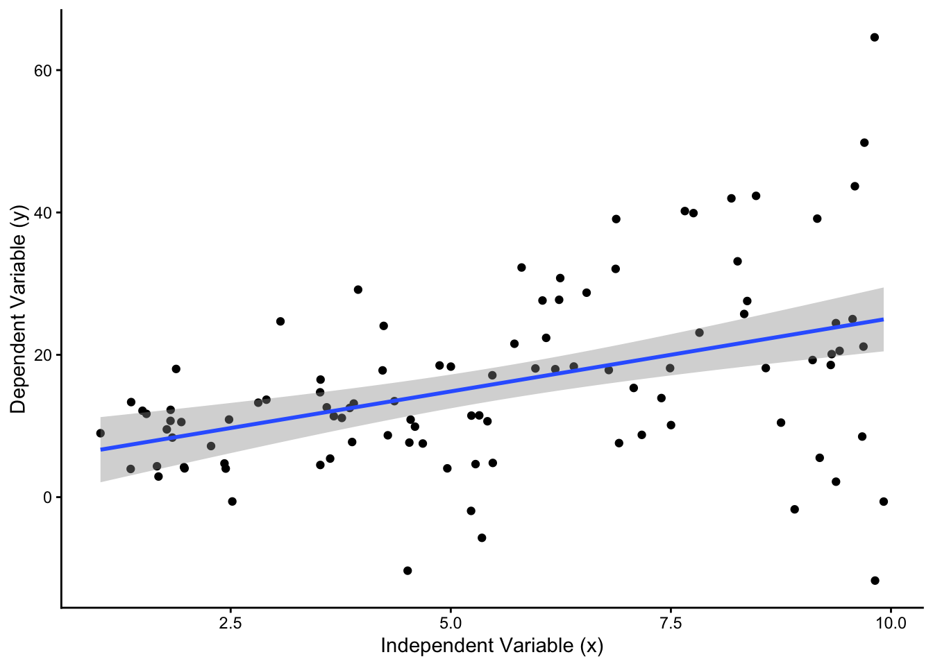
This assumption is violated if some observations are systematically less well explained by the model than others. The graph on the right in Figure 5 depicts this scenario: Here, observations that have higher values on the \(X\) variable are systematically farther away from the regression line than those with low \(X\)-values. This is a case of heteroscedasticity, and a simple regression model will not be appropriate. The problem, simply put, is that a single regression line with a single estimate of the uncertainty around it (here visualized with the gray confidence interval boundaries) is kind of misleading: The confidence interval suggests that there is the same level of uncertainty around the fitted line at low values of \(X\) as at high values of \(X\) - but the underlying data show that this is clearly not the case. Again, when working with a typical survey dataset, heteroscedasticity should not be a problem as long as the model is correctly specified: Sure, some respondents will “fit” the model better and others will be “weirdos”, but there should not be a systematic pattern where some groups of respondents are “weirder” than others.
All this is very different in the case of TSCS data. When working with TSCS data, we can expect three main ways in which the conventional OLS assumptions are violated (see Beck 2001, 274–75):
- Observations are correlated across space (contemporaneous correlation): For example, the economies of Belgium, Luxemburg, and the Netherlands are traditionally closely linked and they trade a lot with each other. This means that if Belgium experiences an economic crisis, then it is very likely that Luxemburg and the Netherlands also experience one at the same time. The same is usually true when it comes to the Nordic countries, to the USA and Canada, or to Germany, Austria, and Switzerland. In practice, this means that the individual data points in a TSCS dataset that covers these countries depend on (i.e., are correlated with) each other.
- Observations are correlated over time (serial correlation): The value of many variables at any given point in time depends strongly on their value in previous years. For example, the unemployment rate in Germany in 1994 is not a random number but depends on the unemployment rate in 1993 and, but less so, that in 1992.
- A given regression model (and the underlying theory) will fit some countries better than others. For example, the US are often somewhat of an outlier when it comes to firearms and gun control because of its very powerful pro-firearm lobby. Therefore, while an increase in gun violence would trigger a restriction of gun laws in most countries, it might have less of an effect in the US. Therefore, if we regress a measure of gun control rules on a measure of gun violence in different countries, then the model will fit the US less well. This, in turn, means that the error terms (or residuals) in that regression models are systematically larger for the US than for other countries. This is called panel heteroscedasticity.
Solution, part 1: Panel-corrected standard errors
Beck and Katz (1995, 1996) have developed a method to deal with the first and third issue, contemporaneous correlation and panel heteroscedasticity: panel-corrected standard errors (PCSEs). Very simply put, this is a specific way to calculate the standard errors (SEs) for regression coefficients and, by implication, any confidence intervals or p-values based on those SEs. This method has quickly become standard practice in the field, and it is now the default way to work with TSCS data.
Obviously, you do not have to calculate PCSEs by yourself. PCSEs have been implemented in two R packages, one of which is called pcse (Bailey and Katz 2011) and the other being the lmtest package, that works together with the plm package from earlier. We will go over an example of how this looks like in practice below.
Solution, part 2: Lagged dependent variables
To deal with the second issue, serial correlation, researchers nowadays use lagged dependent variables (LDVs) in their models. This is less complicated than it may sound: You take your dependent variable and create a “lagged” version of it. This lagged version simply reflects the value of the dependent variable in the previous year.
For example, let’s say that your dependent variable is the unemployment rate and you have data for different countries from 1960 onward. The regular unemployment rate variable will reflect the level of unemployment in any given year and its lag will always show the unemployment rate in the previous year.
The table below illustrates this for the country of Norway: Here, the unemployment rate was 1.2% in 1960, 0.9% in 1961, and 1% in 1962.9 The lagged unemployment rate was 1.2% in 1961 and 0.9% in 1962, reflecting the values from the two respective previous years. The value for 1960 is missing, because the data begin in 1960 and we therefore do not know what the level of unemployment was in 1959. We will go over how to construct this variable with functions from the tidyverse further below.
# A tibble: 10 × 4
   country  year unemp lag_unem
   <chr>   <dbl> <dbl>    <dbl>
 1 Norway   1960   1.2     NA
 2 Norway   1961   0.9      1.2
 3 Norway   1962   1        0.9
 4 Norway   1963   1.3      1
 5 Norway   1964   1.1      1.3
 6 Norway   1965   0.9      1.1
 7 Norway   1966   0.8      0.9
 8 Norway   1967   0.7      0.8
 9 Norway   1968   1.1      0.7
10 Norway   1969   1.1      1.1
Using a LDV in a fixed-effects model is a bit controversial. There is an older study that showed that doing so skews the results, and that this skew paradoxically becomes more severe the more cross-sectional units (e.g., countries) one has (Nickell 1981). Economists have since developed very sophisticated techniques to solve this problem, but these have their own weaknesses (Arellano and Bond 1991; Arellano and Bover 1995; Blundell and Bond 1998).
Beck & Katz (1996; 2011) have long argued in favor of using an LDV to correct for serial correlation in the data, and they have shown that the problem is much less serious than often believed, especially if one works with data that go over many time periods. Specifically, they have shown that you can combine an LDV and a fixed-effects model as long as your dataset covers more than 20 time periods (e.g., years) per country (Beck 2011, 342).
Putting it all together: An applied example
We have now gone over all the issues and complications connected to a regression analysis with TSCS data:
- The fact that we are working with two types of variation, cross-sectional and longitudinal, at the same time
- The fact that this can lead to misleading conclusions about relationships within the data (Simpson’s Paradox)
- Different types of models that focus on different types of variation in the data
- Additional estimation problems (serial correlation, panel-heteroscedasticity) and how to solve them
In the final part, we will do an analysis with a real research dataset, the Comparative Political Data Set (Armingeon et al. 2024), to see how all of these different things come together in an actual research project.
The dependent variable will be the amount of social security transfers (e.g., sickness or unemployment benefits, family allowances), which can be seen as a measure of the size of the welfare state (e.g., Castles and Obinger 2007).10 We measure this with the sstran variable from the CPSD. This variable has the advantage that it is available from 1960 onwards for many countries, in contrast to other spending variables (like the one on pensions we used above), which are only available from 1980 onward.
Our independent variables are based on a few leading explanations for welfare state development:
ud: The strength of trade unions, measured as the share of union members in the working population, reflecting Power Resources Theory (Korpi 1989)realgdpgr: The economic growth rate (real GDP growth, in %), which reflects the more “functionalist” perspective that welfare state spending goes up when there is an economic downturn and more people need support from the government (e.g., Wilensky and Lebeaux 1958)elderly: The share of persons that are older than 65 in the population, which also reflects the functionalist perspectiveopenc: The openness of the economy, measured as the amount of trade (the sum of exports and imports) as a share of GDP. Including this allows us to test the theory that economic globalization has either a positive (Cameron 1978; Walter 2010) or a negative (Cerny 1997; Genschel 2002) effect on the welfare statewomenpar: The share of female members of parliament. This reflects the theory that a better representation of women in politics could have effects on the welfare state (e.g., Iversen and Rosenbluth 2010; Morgan 2013).prop: The type of electoral system (single-member district vs. proportional representation), reflecting the theory that political institutions affect welfare state development (Iversen and Soskice 2006)
The CPDS dataset covers both the “traditional” Western democracies of Europe, North America, and Australasia, but also the formerly communist countries of Central and Eastern Europe. Unfortunately, since the latter were not real democracies before 1990, the CPDS covers them only after 1990 or in some cases 1995. This means that our “panel” of countries is “unbalanced”: We have more observations for some countries than for others. This is not a massive problem, but it is generally preferrable to have “balanced” panel data (see Bailey and Katz 2011, sec. 3.2). To keep things simple, we focus the analysis on the “traditional” Western countries.
Model selection
Most of the independent variables vary over time, but we know that the prop variable does not (or only in a few instances). This should inform our modelling strategy. Specifically, to model the effect of a stable political institution like the electoral system, we should use a between-effects model. Since this model basically eliminates the time-dimension in the data and corresponds to a regular OLS estimation, we do not need to worry about lagged dependent variables or different types of standard errors.
When it comes to the other variables, we need to make sure that we are not running into Simpson’s Paradox and confuse stable differences between countries with over-time changes within countries. The fixed-effects or “within” model is a reasonable choice here. In this case, we actively use the time-dimension in the dataset, which means we need to deal with the problem of serial correlation in the data. We do this by including a lagged dependent variable as a predictor into the model (Beck and Katz 1996). In addition, we follow standard practice and convert the standard errors to PCSEs (Beck and Katz 1995).
Data management
Creating a lagged dependent variable
The first thing we want to do is to create a lagged dependent variable. We can do this with the lag() function from dplyr within mutate(). In this case, it makes sense to be explicit in our code that we want to use the lag() function from dplyr because there are other packages that also have functions called lag() and which sometimes work a bit differently. We want to be sure we use the correct function. The CPDS dataset should normally be sorted by country and year, but manually sorting it again is easy (and getting this wrong is costly), so we do that before creating the lag. We also need to make sure to group the data by country. Otherwise, the last observation from one country would become the lag for the following country, which is obviously not what we want.
The code below does all this in one swoop: It sorts and groups the data, creates the lag, and ungroups the data again:
cpds |>
  arrange(country,year) |>
  group_by(country) |>
  mutate(lag_sstran = dplyr::lag(sstran)) |>
  ungroup() -> cpds
Dummy-coding the electoral system variable
Next, we change the prop variable a bit. It is saved as a numeric variable in the dataset, but since the type of electoral system is fundamentally a categorical variable, it should also be stored in R as one (i.e., as a factor). Also, the original prop variable has three categories (0 for “single member district”, 1 for “modified proportional”, 2 for “proportional”) and it makes sense to group the first two categories together to be more in line with the analysis by Iversen & Soskice (2006).
Here, we use if_else() to create a dummy variable called elsys that distinguishes proportional (“PR”) versus majoritarian (“SMD”) electoral systems
cpds |>
  mutate(elsys = if_else(prop==2,"PR","SMD")) -> cpds
Selecting relevant countries
Finally, we limit the analysis to the “traditional” Western democracies. To do so, we use a variable called cpds1, which indicates the countries that were covered in the original version of the CPDS dataset – which were only the countries we are interested in here:
cpds |>
  filter(cpds1 == 1) -> cpds
Between-effects analysis
We start the regression analysis with the simplest part, the between-effects model to test the effect of the electoral system on social security transfers. As shown earlier, we use the plm() function with the model set to “between”:
be <- plm(sstran ~ elsys,
          data = cpds,
          index = c("country","year"),
          model = "between")
summary(be)
Oneway (individual) effect Between Model
Call:
plm(formula = sstran ~ elsys, data = cpds, model = "between",
index = c("country", "year"))
Unbalanced Panel: n = 23, T = 45-62, N = 1363
Observations used in estimation: 23
Residuals:
Min. 1st Qu. Median 3rd Qu. Max.
-7.27390 -1.24600 0.22216 1.49289 6.52699
Coefficients:
Estimate Std. Error t-value Pr(>|t|)
(Intercept) 13.67514 0.72446 18.8762 1.188e-14 ***
elsysSMD -3.01171 1.37756 -2.1863 0.04026 *
---
Signif. codes: 0 '***' 0.001 '**' 0.01 '*' 0.05 '.' 0.1 ' ' 1
Total Sum of Squares: 213.93
Residual Sum of Squares: 174.26
R-Squared: 0.18541
Adj. R-Squared: 0.14662
F-statistic: 4.77972 on 1 and 21 DF, p-value: 0.040261We find that countries with majoritarian electoral systems spend on average around 3% less of their GDP on social security transfers than countries with proportional representation systems. This is in line with the findings by Iversen & Soskice (2006). Notice also the information about the data that went into the model. In principle, the dataset includes 1363 (valid) observations, but the model aggregates them to 23 country-by-country average values that are actually used in the estimation.
Fixed-effects analysis
Next, we move to the more complex part of the analysis where we use the fixed effects model. Just to show again that there are different ways of getting to the correct results, we specify this model in three ways: as a regular OLS model (with lm()) including country dummies, as a “pooling” model with plm() also including country dummies, and as a “within” model with plm() that does not include country dummies. All models include the lagged dependent variable that we created earlier
ols <- lm(sstran ~ lag_sstran + realgdpgr + ud + openc + elderly + womenpar + factor(country),
           data = cpds)

pool <- plm(sstran ~ lag_sstran + realgdpgr + ud + openc + elderly + womenpar + factor(country),
           data = cpds,
           index = c("country","year"),
           model = "pooling")

fe <- plm(sstran ~ lag_sstran + realgdpgr + ud + openc + elderly + womenpar,
           data = cpds,
           index = c("country","year"),
           model = "within")

screenreg(list(ols,pool,fe),
          custom.model.names = c("OLS w. country dummies","Pooling w. country dummies","Within model"))
===============================================================================================
                               OLS w. country dummies  Pooling w. country dummies  Within model
-----------------------------------------------------------------------------------------------
(Intercept)                       1.31 ***                1.31 ***
                                 (0.20)                  (0.20)
lag_sstran                        0.90 ***                0.90 ***                    0.90 ***
                                 (0.01)                  (0.01)                      (0.01)
realgdpgr                        -0.18 ***               -0.18 ***                   -0.18 ***
                                 (0.01)                  (0.01)                      (0.01)
ud                                0.01 **                 0.01 **                     0.01 **
                                 (0.00)                  (0.00)                      (0.00)
openc                            -0.00 ***               -0.00 ***                   -0.00 ***
                                 (0.00)                  (0.00)                      (0.00)
elderly                          -0.01                   -0.01                       -0.01
                                 (0.01)                  (0.01)                      (0.01)
womenpar                         -0.00                   -0.00                       -0.00
                                 (0.00)                  (0.00)                      (0.00)
factor(country)Austria            1.02 ***                1.02 ***
                                 (0.16)                  (0.16)
factor(country)Belgium            1.00 ***                1.00 ***
                                 (0.17)                  (0.17)
factor(country)Canada             0.22                    0.22
                                 (0.14)                  (0.14)
factor(country)Denmark            0.61 ***                0.61 ***
                                 (0.17)                  (0.17)
factor(country)Finland            0.62 ***                0.62 ***
                                 (0.17)                  (0.17)
factor(country)France             1.18 ***                1.18 ***
                                 (0.19)                  (0.19)
factor(country)Germany            0.89 ***                0.89 ***
                                 (0.16)                  (0.16)
factor(country)Greece             0.28                    0.28
                                 (0.22)                  (0.22)
factor(country)Iceland           -0.39                   -0.39
                                 (0.24)                  (0.24)
factor(country)Ireland            0.91 ***                0.91 ***
                                 (0.17)                  (0.17)
factor(country)Italy              0.81 ***                0.81 ***
                                 (0.15)                  (0.15)
factor(country)Japan              0.40 **                 0.40 **
                                 (0.15)                  (0.15)
factor(country)Luxembourg         1.95 ***                1.95 ***
                                 (0.29)                  (0.29)
factor(country)Netherlands        0.94 ***                0.94 ***
                                 (0.17)                  (0.17)
factor(country)New Zealand        0.39 *                  0.39 *
                                 (0.16)                  (0.16)
factor(country)Norway             0.64 ***                0.64 ***
                                 (0.15)                  (0.15)
factor(country)Portugal           0.44 *                  0.44 *
                                 (0.20)                  (0.20)
factor(country)Spain              0.82 ***                0.82 ***
                                 (0.17)                  (0.17)
factor(country)Sweden             0.52 **                 0.52 **
                                 (0.18)                  (0.18)
factor(country)Switzerland        0.42 **                 0.42 **
                                 (0.15)                  (0.15)
factor(country)United Kingdom     0.42 **                 0.42 **
                                 (0.14)                  (0.14)
factor(country)USA                0.43 *                  0.43 *
                                 (0.17)                  (0.17)
-----------------------------------------------------------------------------------------------
R^2                               0.97                    0.97                        0.94
Adj. R^2                          0.97                    0.97                        0.94
Num. obs.                      1129                    1129                        1129
===============================================================================================
*** p < 0.001; ** p < 0.01; * p < 0.05
The table at the end shows that we get the exact same results regardless of which specification we use. The only difference is that the first two models include an intercept and, obviously, coefficients for the country dummy variables.
Before we interpret the results, we first have to correct the standard errors. The results above use the regular OLS standard errors, which can be misleading. To fix this issue, we calculate PCSEs using the Beck & Katz (1995) procedure as described above.
This procedure is implemented in the lmtest package, which is directly compatible with the plm package (Millo 2017). The package can be installed via CRAN with install.packages() and then loaded with library():
# install.packages("lmtest")
library(lmtest)
Loading required package: zoo
Attaching package: 'zoo'The following objects are masked from 'package:base':
as.Date, as.Date.numericWe use the coeftest() function from the package to convert the standard errors from the “within” model (fe). We specify that we want the Beck/Katz correction with vcovBK, that the data should be clustered by time (this makes sure that we really correct for panel-heteroscedasticity and not for serial correlation). The rest follows the example of Urdinez & Cruz (2020, 171). We save the corrected results as pcse and can then use screenreg() to directly compare the original and corrected results (or, later, to present the results in a table):
pcse <- coeftest(fe, vcov = vcovBK, type = "HC1", cluster = "time")

screenreg(list(fe,pcse), digits = 3, stars = 0.05,
          custom.model.names = c("Within model","Within model (PCSE)"))
=============================================
            Within model  Within model (PCSE)
---------------------------------------------
lag_sstran     0.904 *     0.904 *
              (0.009)     (0.013)
realgdpgr     -0.180 *    -0.180 *
              (0.009)     (0.011)
ud             0.008 *     0.008 *
              (0.003)     (0.003)
openc         -0.004 *    -0.004 *
              (0.001)     (0.001)
elderly       -0.013      -0.013
              (0.012)     (0.012)
womenpar      -0.000      -0.000
              (0.003)     (0.004)
---------------------------------------------
R^2            0.938
Adj. R^2       0.936
Num. obs.   1129
=============================================
* p < 0.05
If you take a careful look at the standard errors under the coefficients, you notice that the PCSEs are generally a bit larger than the original ones. For example, the SE for the coefficient of the lagged dependent variable goes up from 0.009 to 0.013, and the SE for the coefficient on real GDP growth increases from 0.009 to 0.011.
Now we can interpret the results: The lagged dependent variable indicates the extent of serial correlation in the dependent variable, which is clearly high (0.9) and statistically significant. GDP growth has a significant and negative effect, which means that every additional percent GDP growth lowers spending on social security transfers by 0.18 percentage points. This makes sense: More economic growth means fewer people who are unemployed or otherwise financially in trouble, which lowers spending on the welfare state.
The strength of trade unions (ud) has a small but positive effect, which indicates that every additional percent of trade union members in the economically active population increases social security spending by 0.01 percentage points. We also find a significant negative effect of greater economic openness, but this effect is very, very small. Interestingly, the share of elderly in the population and the share of female members of parliament do not have significant effects.
Conclusion
This was one of the longer posts in this blog and, to be fair, the issues and methods we covered here are a bit more advanced than a standard linear regression. Still, you should ideally have taken away that seemingly cryptic methods like “within” or “between” estimations are really not that complicated: They are just different ways of “slicing” a panel or TSCS dataset to extract different forms of variation and co-variation in the data. Adjusting regression standard errors is also, strictly speaking, a quite technical affair, but we do have software that does this for us with a few lines of code and thus makes this easy for those of us who are willing to trust the experts.
You now have the basic skills you need to conduct your own TSCS regression analyses, at least as long as your dependent variable is numeric. You might, of course, also run into a situation where you work with TSCS data but your dependent variable is binary (e.g., “peace” vs. “war”). In that case, you can refer to the articles by Beck et al. (1998) and Carter & Signorino (2010). The first shows that you can use logistic regression (glm()) to analyze these data as long as you account for the temporal dynamics in the data. The second article shows that you can do that very easily by simply including different polynomials of time into your model. For example, if your time-variable is called year, then your model specification will be:
mod <- glm(dummy_var ~ indepvars + year + I(year^2) + I(year^3),
           data = your_dataset,
           family = binomial(link = "logit"))
summary(mod)
You may also get to a point where you want to study over-time dynamics in your data more systematically, for example to see if some variables have both short-term and long-term effects and over which time horizon the long-term effects really work. If that is the case, you can read the articles by DeBoef & Keele (2008) and Beck & Katz (2011), who explain how you can model these things with TSCS data. You should now have the necessary background to understand how to implement the models they suggest in practice.
References
Adema, Willem, and Maxime Ladaique. 2009. “How Expensive Is the Welfare State?: Gross and Net Indicators in the OECD Social Expenditure Database (SOCX).” OECD Social, Employment and Migration Working Papers 92.
Arellano, Manuel, and Stephen Bond. 1991. “Some Tests of Specification for Panel Data: Monte Carlo Evidence and an Application to Employment Equations.” The Review of Economic Studies 58 (2): 277–97.
Arellano, Manuel, and Olympia Bover. 1995. “Another Look at the Instrumental Variable Estimation of Error-Components Models.” Journal of Econometrics 68 (1): 29–51.
Armingeon, Klaus, Sarah Engler, Lucas Leemann, and David Weisstanner. 2024. Comparative Political Data Set 1960-2022. University of Zurich, Leuphana University Lueneburg,; University of Lucerne.
Bailey, Delia, and Jonathan N. Katz. 2011. “Implementing Panel Corrected Standard Errors in R: The pcse Package.” Journal of Statistical Software 42 (CS1): 1–11.
Beck, Nathaniel. 2001. “Time-Series-Cross-Section Data: What Have We Learned in the Past Few Years?” Annual Review of Political Science 4: 271–93.
Beck, Nathaniel. 2008. “Time-Series Cross-Section Methods.” In The Oxford Handbook of Political Methodology, edited by Janet M. Box-Steffensmeier, Henry E. Brady, and David Collier. Oxford University Press.
Beck, Nathaniel. 2011. “Of Fixed-Effects and Time-Invariant Variables.” Political Analysis 19 (2): 119–22.
Beck, Nathaniel, Kristian Skrede Gleditsch, and Kyle Beardsley. 2006. “Space Is More Than Geography: Using Spatial Econometrics in the Study of Political Economy.” International Studies Quarterly 50 (1): 27–44.
Beck, Nathaniel, and Jonathan N. Katz. 1995. “What to Do (and Not Do Do) with Time-Series Cross-Section Data.” American Political Science Review 89 (3): 634–47.
Beck, Nathaniel, and Jonathan N. Katz. 1996. “Nuisance Vs. Substance: Specifying and Estimating Time-Series-Cross-Section Models.” Political Analysis 6 (1): 1–36.
Beck, Nathaniel, Jonathan N. Katz, and Richard Tucker. 1998. “Taking Time Seriously: Time-Series-Cross-Section Analysis with a Binary Dependent Variable.” American Journal of Political Science 42 (4): 1260–88.
Blundell, Richard, and Stephen Bond. 1998. “Initial Conditions and Moment Restrictions in Dynamic Panel Data Models.” Journal of Econometrics 87 (1): 115–43.
Bonoli, Giuliano. 2001. “Political Institutions, Veto Points, and the Process of Welfare State Adaptation.” In The New Politics of the Welfare State, edited by Paul Pierson. Oxford University Press.
Box-Steffensmeier, Janet M., John R. Freeman, Matthew P. Hitt, and Jon C. Pevehouse. 2014. Time Series Analysis for the Social Sciences. Cambridge University Press.
Box-Steffensmeier, Janet, and Agnar Freyr Helgason. 2016. “Introduction to Symposium on Time Series Error Correction Methods in Political Science.” Political Analysis 24 (1): 1–2.
Brady, David, Jason Beckfield, and Martin Seeleib-Kaiser. 2005. “Economic Globalization and the Welfare State in Affluent Democracies, 1975-2001.” American Sociological Review 70 (6): 921–48.
Burgoon, Brian. 2001. “Globalization and Welfare Compensation: Disentangling the Ties That Bind.” International Organization 55 (3): 509–51.
Cameron, David R. 1978. “The Expansion of the Public Economy: A Comparative Analysis.” American Political Science Review 72 (4): 1243–61.
Carter, David B., and Curtis S. Signorino. 2010. “Back to the Future: Modeling Time Dependence in Binary Data.” Political Analysis 18 (3): 271–92.
Castles, Francis G., and Herbert Obinger. 2007. “Social Expenditure and the Politics of Redistribution.” Journal of European Social Policy 17 (3): 206–22.
Cerny, Philip G. 1997. “Paradoxes of the Competition State: The Dynamics of Political Globalization.” Government and Opposition 32 (2): 251–74.
Croissant, Yves, and Giovanni Millo. 2008. “Panel Data Econometrics in R: The plm Package.” Journal of Statistical Software 27 (2): 1–43.
De Boef, Suzanna, and Luke Keele. 2008. “Taking Time Seriously.” American Journal of Political Science 52 (1): 184–200.
Enns, Peter K, Nathan J. Kelly, Takaaki Masaki, and Patrick C. Wohlfarth. 2016. “Don’t Jettison the General Error Correction Model Just yet: A Practical Guide to Avoiding Spurious Regression with the GECM.” Research & Politics 3 (2): 1–13.
Esping-Andersen, Gøsta. 1990. The Three Worlds of Welfare Capitalism. Polity Press.
Garrett, Geoffrey, and Deborah Mitchell. 2001. “Globalization, Government Spending and Taxation in the OECD.” European Journal of Political Research 39 (2): 145–77.
Genschel, Philipp. 2002. “Globalization, Tax Competition, and the Welfare State.” Politics & Society 30 (2): 245–75.
Grant, Taylor, and Matthew J. Lebo. 2016. “Error Correction Methods with Political Time Series.” Political Analysis 24 (1): 3–30.
Heiss, Florian. 2020. Using R for Introductory Econometrics. 2nd ed. Düsseldorf.
Huber, Evelyne, Charles Ragin, and John D. Stephens. 1993. “Social Democracy, Christian Democracy, Constitutional Structure, and the Welfare State.” American Journal of Sociology 99 (3): 711–49.
Huber, Evelyne, and John D. Stephens. 2000. “Partisan Governance, Women’s Employment, and the Social Democratic Service State.” American Sociological Review 65 (3): 323–42.
Huber, Evelyne, and John D. Stephens. 2001. Development and Crisis of the Welfare State. Chicago University Press.
Immergut, Ellen M. 1990. “Institutions, Veto Points, and Policy Results: A Comparative Analysis of Health Care.” Journal of Public Policy 10 (4): 391–416.
Immergut, Ellen M. 1992. Health Politics: Interests and Institutions in Western Europe. Cambridge University Press.
Iversen, Torben, and Thomas R. Cusack. 2000. “The Causes of Welfare State Expansion: Deindustrialization or Globalization?” World Politics 52 (3): 313–49.
Iversen, Torben, and Frances Rosenbluth. 2010. Women, Work, & Politics: The Political Economy of Gender Inequality. Yale University Press.
Iversen, Torben, and David Soskice. 2006. “Electoral Institutions and the Politics of Coalitions: Why Some Democracies Redistribute More Than Others.” American Political Science Review 100 (2): 165–81.
Kellstedt, Paul M, and Guy D Whitten. 2018. The Fundamentals of Political Science Research. Cambridge University Press.
Korpi, Walter. 1989. “Power, Politics, and State Autonomy in the Development of Social Citizenship: Social Rights During Sickness in Eighteen OECD Countries Since 1930.” American Sociological Review 54 (3): 309–28.
Lebo, Matthew J., and Patrick W. Kraft. 2017. “The General Error Correction Model in Practice.” Research & Politics 4 (2): 1–13.
Leifeld, Philip. 2013. “Texreg: Conversion of Statistical Model Output in r to LATEX and HTML Tables.” Journal of Statistical Software 55 (8): 1–24.
Lindberg, Staffan I, Michael Coppedge, John Gerring, and Jan Teorell. 2014. “V-Dem: A New Way to Measure Democracy.” Journal of Democracy 25 (3): 159–69.
Millo, Giovanni. 2017. “Robust Standard Error Estimators for Panel Models: A Unifying Approach.” Journal of Statistical Software 82: 1–27.
Morgan, Kimberly J. 2013. “Path Shifting of the Welfare State: Electoral Competition and the Expansion of Work-Family Policies in Western Europe.” World Politics 65 (1): 73–115.
Murray, Michael P. 1994. “A Drunk and Her Dog: An Illustration of Cointegration and Error Correction.” The American Statistician 48 (1): 37–39.
Nickell, Stephen. 1981. “Biases in Dynamic Models with Fixed Effects.” Econometrica 49 (6): 1417–26.
Obama, Barack. 2016. “United States Health Care Reform. Progress to Date and Next Steps.” Journal of the American Medical Association 316 (5): 525–32.
Obinger, Herbert. 2002. “Föderalismus und wohlfahrtsstaatliche Entwicklung. Österreich und die Schweiz im Vergleich.” Politische Vierteljahresschrift 43 (2): 235–71.
Plümper, Thomas, and Vera E. Troeger. 2007. “Efficient Estimation of Time-Invariant and Rarely Changing Variables in Finite Sample Panel Analysis with Unit Fixed Effects.” Political Analysis 15 (2): 124–39.
Plümper, Thomas, Vera E. Troeger, and Philip Manow. 2005. “Panel Data Analysis in Comparative Politics: Linking Method to Theory.” European Journal of Political Research 44 (2): 327–254.
Sassen, Saskia. 1996. Losing Control?: Sovereignty in the Age of Globalization. Columbia University Press.
Stimson, James A. 1985. “Regression in Space and Time: A Statistical Essay.” American Journal of Political Science 29 (4): 914–47.
Swank, Duane. 2001. “Political Institutions and Welfare State Restructuring: The Impact of Institutions on Social Policy Change in Developed Democracies.” In The New Politics of the Welfare State, edited by Paul Pierson. Oxford University Press.
Tsebelis, George. 2002. Veto Players: How Political Institutions Work. Princeton University Press.
Urdinez, Francisco, and Andres Cruz. 2020. R for Political Data Science: A Practical Guide. CRC Press.
Walter, Stefanie. 2010. “Globalization and the Welfare State: Testing the Microfoundations of the Compensation Hypothesis.” International Studies Quarterly 54 (2): 403–26.
Wilensky, Harold L., and Charles Nathan Lebeaux. 1958. Industrial Society and Social Walfare: The Impact of Industrialization on the Supply and Organization of Social Welfare Services in the United States. Russell Sage.
Wilson, Sven E., and Daniel M. Butler. 2007. “A Lot More to Do: The Sensitivity of Time-Series Cross-Section Analyses to Simple Alternative Specifications.” Political Analysis 15 (2): 101–23.
Footnotes
The discussion among political science methodologists on how to correctly analyze TSCS data was strongly based on techniques for panel data analysis (see Beck 2001, 2011, 2008, 2011; Beck and Katz 1995, 1996; Beck et al. 1998, 2006; Stimson 1985; Plümper et al. 2005; Plümper and Troeger 2007; De Boef and Keele 2008; Wilson and Butler 2007, Kittel1999, Kittel2005).↩︎
De Doef & Keele (2008) and Beck & Katz (2011) show how you can deal with non-stationary variables in a regression analysis (see also Box-Steffensmeier and Helgason 2016; Enns et al. 2016; Grant and Lebo 2016; Lebo and Kraft 2017).↩︎
I saved the dataset as
cpds_2024.dta. You might have saved it under a different name, in which case you obviously need to adjust that in your code.↩︎I used ChatGPT to generate this graph.↩︎
The main complicating factor is that TSCS data also have many of the characteristics of longer time series, meaning trends and the above-mentioned degrees of stationarity or integration. This means that analysts also have to think about how to model these features of the data Beck (2011). This is less of a problem when working with “shorter” panel data.↩︎
You might remember that we make a similar adjustment when we calculate the standard deviation of a variable, where we also “use up” information in the first step by calculating the variable’s mean (Kellstedt and Whitten 2018, 137).↩︎
As Wilson and Butler (2007, 108) point out, the between-effects is in these cases an “honest” model because it does not artificially inflate the number of observations in your dataset.↩︎
The data are from (Armingeon et al. 2024).↩︎
Although not necessarily its degree of “decommodification” (Esping-Andersen 1990).↩︎
Citation
BibTeX citation:
@online{knotz2026,
  author = {Knotz, Carlo},
  title = {Regression Analyses with Macro-Level Data},
  date = {2026-01-26},
  url = {https://cknotz.github.io/getstuffdone_blog/posts/tscs_regs/},
  langid = {en}
}
For attribution, please cite this work as:
Knotz, Carlo. 2026. “Regression Analyses with Macro-Level
Data.” January 26. https://cknotz.github.io/getstuffdone_blog/posts/tscs_regs/.