R version 4.4.1 (2024-06-14) -- "Race for Your Life"
Copyright (C) 2024 The R Foundation for Statistical Computing
Platform: x86_64-apple-darwin20

R is free software and comes with ABSOLUTELY NO WARRANTY.
You are welcome to redistribute it under certain conditions.
Type 'license()' or 'licence()' for distribution details.

  Natural language support but running in an English locale

R is a collaborative project with many contributors.
Type 'contributors()' for more information and
'citation()' on how to cite R or R packages in publications.

Type 'demo()' for some demos, 'help()' for on-line help, or
'help.start()' for an HTML browser interface to help.
Type 'q()' to quit R.Tutorial 0: Installation & Setup
1 Introduction
To successfully complete the Kvantitativ forskningsmetode course, you need to work with R and RStudio.
This tutorial introduces you to R and RStudio and shows you how you install these applications on your computer and set everything up so that you are ready to do analyses.
Hvis du ønsker å lese en norsk tekst i tillegg: Hermansen, S. S. (2019). Lær deg R: En innføring i statistikkprogrammets muligheter Fagbogforlaget, Bergen, kapittel 1 & 4.1
1.1 About R
R is one of the most popular software tools for data analysis and data science. R can be used for “traditional” quantitative data analysis (e.g., regression analysis), but also much more: Quantitative text analysis, web scraping, interactive data visualization, Big Data analysis, and machine learning.
R is what professional data analysts, data scientists, and researchers use in their work. It is used in academia, but also in the private sector or the media (e.g., news channels like the BBC and companies like YouGov, Netflix, or Meta/Facebook).1 Therefore, knowing how to work with R is a big advantage when you look for jobs — and this is one reason for why we want you to learn it.
R is also a really good tool to have for your studies. The work for your BA and perhaps MA thesis will get considerably easier if you are able to quickly download and analyze a dataset — no hours of transcribing interviews or digging through dusty archives.
R looks and works also quite similarly to other widely used tools like Python and Javascript. This means that learning Python or Javascript becomes a lot easier and quicker if you already know at least a bit of R.
Last but not least, R is open-source and free.
Working with R means writing computer code — again, just like Python or Javascript. You will not be able to run your analyses by clicking your way through menus or dragging and dropping things around, as you would do when working with Microsoft Word etc. Obviously, this may come as quite a change for you and may even feel strange.
But: R can be learned. Others have done it before, and there are many who start using R who have no prior experience with programming or computer languages. Still, it might take some time before you are really used to it.
Think about learning R like learning a foreign language: The start is often very confusing, and things that are really simple feel really difficult. The trick to getting better is to just keep practicing and not giving up. If you do that, you will soon feel that you are making progress!
1.2 About RStudio
Working with R has become quite a bit easier with the arrival of RStudio a while ago. Where R by itself gives you only a bland and empty computer code Console and an output window to work with, RStudio provides you with a more comfortable interface (or “integrated development environment”, IDE, to use the official term) that shows you which datasets and variables you are currently working with, gives you direct access to help files, and helps you with many other tasks (but you will still have to write code!). The basic version of RStudio is also open-source and free to use.
2 Installing R & RStudio
You will of course first need to install both R and RStudio before you can use them. You can download R and RStudio from https://posit.co/download/rstudio-desktop/ (no need to go for the pro-versions; the free Desktop version is more than sufficient!).
If you like, you can also watch a video that will guide you through the installation process: https://vimeo.com/415501284. The video is a bit outdated (the website for RStudio is different now), but the most important information is still correct.
R and RStudio!
If your operating system (Windows, MacOS, Linux) is too old to support the latest versions of R and RStudio, then you have to update your operating system first.
Yes, this is absolutely necessary. Many of the procedures and tools that you need to use during this course work only with the latest versions of R and RStudio.
3 Your first steps in R & RStudio
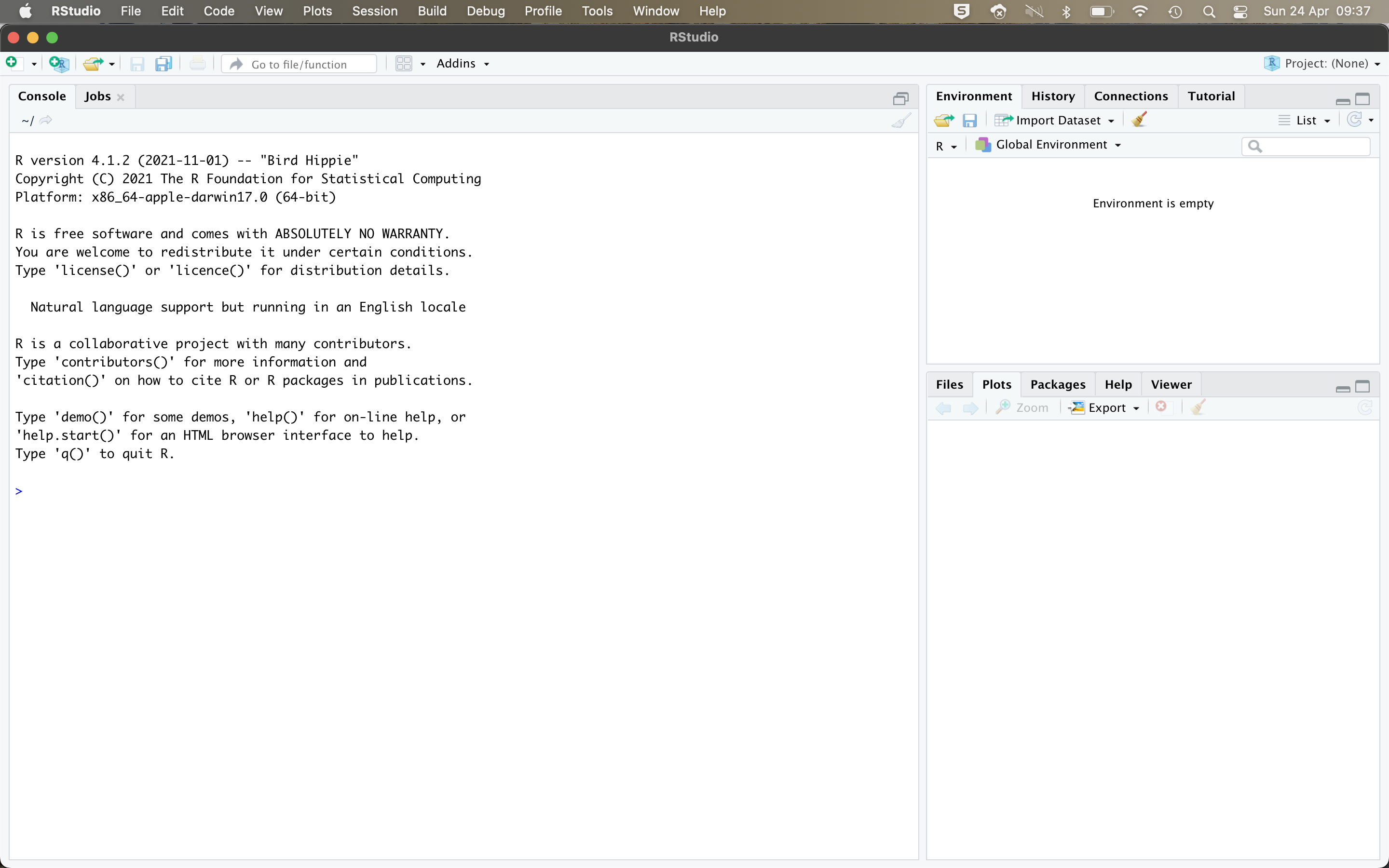
When you are done with the installation, open RStudio. You should now see the RStudio interface pop up on your screen, which should look like the screenshot below:
3.1 What you see
Let’s quickly go over what you are seeing:
- The large window on the left is the Console. This is where you can enter your commands and this is also where your results (other than graphs) will be shown (you can ignore the other tabs for now).
- The smaller window in the upper right corner shows you your current working environment. It is currently empty but will later show you a list of all the variables, datasets, and other “objects” that are loaded at any given point. (You may also see that this window has other tabs labeled “History”, “Connections”, and “Tutorial”. You can also ignore these for now.)
- The smaller window in the lower right corner is where any graphs (“Plots”) you create later will be shown, and this is also where the “Help” files appear if you request them. (You can also access and open “Files” on your computer, and see a list of add-on packages that you can install. These tabs are also not that important right now.)
You can customize how RStudio looks via the “Options” menu (yes, there is a regular click-based menu!). You can open the “Options” menu via the taskbar at the top (“Tools” -> “Global Options…”). When the menu has popped up, navigate to “Appearance”. You can select a different theme and adjust other settings there.
3.2 Where is R?
You may be wondering why you had to install R when you are now working in RStudio and not in R. Technically, you are already working with R. You can see that written in the output that appears in the Console window. It should read something like:
When you run RStudio, R is running “under the hood”. You can think of RStudio as the instrument panel and steering wheel in a car, and R as the car’s engine.
4 Some housekeeping
4.1 Avoiding chaos
There is one important bit of housekeeping you need to do now to reduce chaos and confusion when working with R.
- Open the main options menu in
RStudio(click on “Tools” in the taskbar at the top, and then open the “Global Options” menu at the bottom of the list). - Under “Workspace” (shown right in the middle of the first page of the menu):
- Untick/deactivate “Restore .RData into workspace at startup”.
- In the dropdown menu next to “Save workspace to .RData on exit”, select “Never”.
Your settings should now look like those in the screenshot below.
When you are done, click “OK” to close the menu.
4.2 Keeping everything organized: Projects and working directories
Once you really start working with R, you will use a lot of different files: Dataset files go into R, and all the different graphs and tables that present the results of your analysis come out again. In addition, you will have one or more code files that document your code (more on that comes below). Obviously, you need to keep an overview over the different files and where they are on your computer.
RStudio offers you a great way to keep all these files organized: Projects. A project automatically organizes all the files you need to work with in a given context (e.g., this course) and makes sure that any outputs you create (e.g., graphs) are stored somewhere where you can find them.
You should have one (and only one) project for this course in RStudio. This project includes all the files (dataset files, code files, output) that you work with during this course. All these files should be stored in one (and only one) folder on your computer. Your project will be associated with that folder.
Follow these steps to create the project:
- Open File Explorer (on Windows) or Finder (on Mac) and create a folder on your computer where you want to store all the
R-related files for this course (for example asDocuments/Uni/3rd_semester/BST290/R_files). - Then go back to
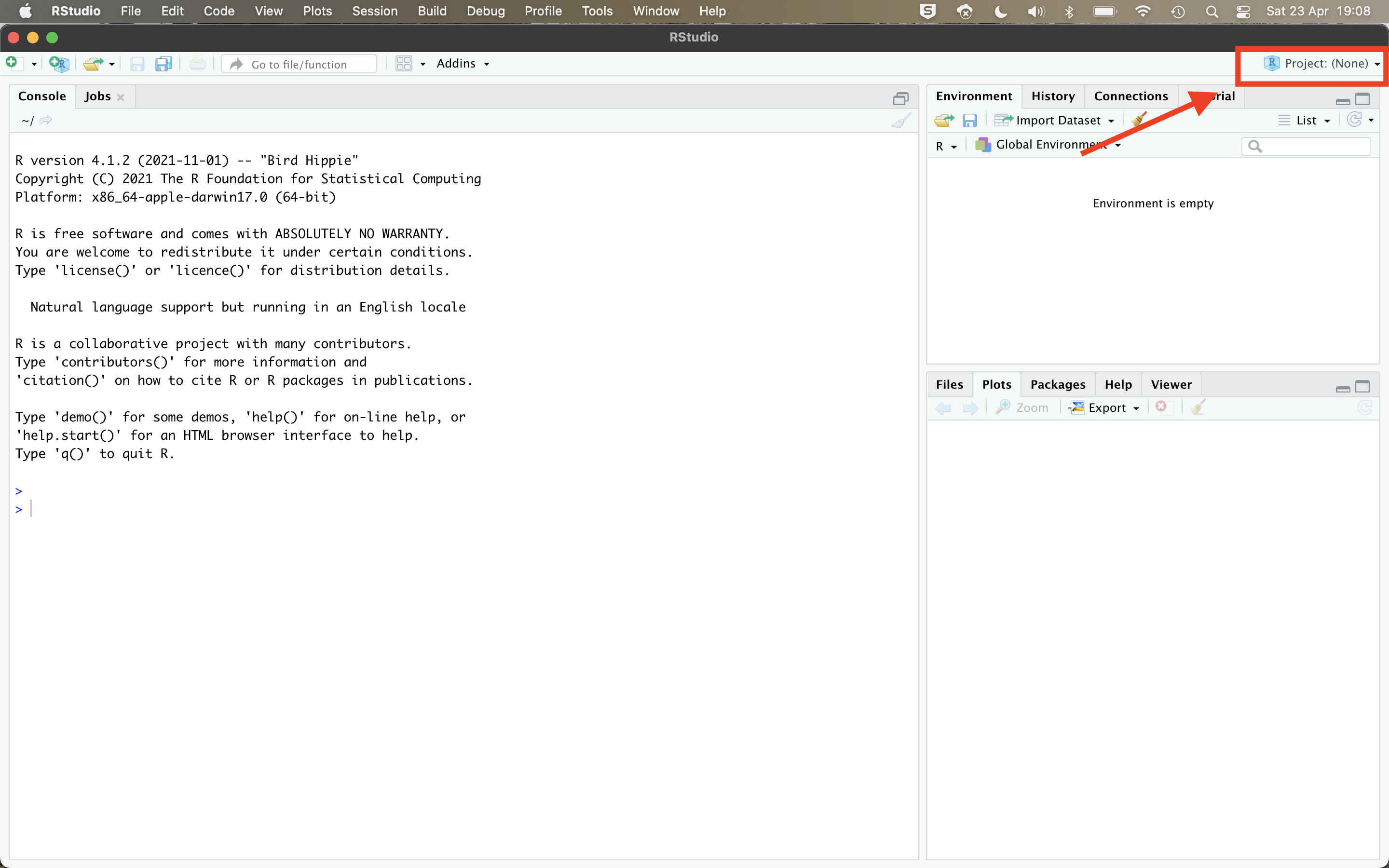
RStudio. If you look at the top right corner of yourRStudiowindow, you should see a little blue box symbol and “Project: (None)” written next to it (see also the screenshot on the following page). This is where you can create and open projects. - Click on that symbol to open a little dropdown menu. Choose New Project…
- In the menu that pops up, choose Existing Directory.
- Use the Browse… button to select the new folder you just created.
- Then click on Create Project.
RStudio will then restart. When it is done restarting, you should see your project name in the upper right of your screen, next to the blue box symbol. This means that you are now working inside your new project folder. Every time you create a new file (e.g., a graph), that file will be saved in this project folder. In other words, this folder is now your “Working Directory”.2
5 Final housekeeping: Installing packages
The final step of this tutorial is to install packages.
R packages are little add-on programs that provide tools and functionalities that R by itself does not have and which make your life a lot easier. You can think of R packages as similar to smartphone apps — extra tools on top of the regular software.
5.1 Installing the tidyverse package
The first package you install is called the tidyverse package. Strictly speaking, the tidyverse is an entire collection of different R packages, but all these packages fit neatly together and are therefore bundled in a “package of packages”.
The tidyverse packages were designed to make things that are often difficult (data import, data cleaning & management, visualization) a lot easier (see also tidyverse.org).
We will use the tidyverse a lot in this course, so it is absolutely necessary that you install it!
You can install the tidyverse directly from the main R “app-store”: The Central R Archive Network or CRAN.
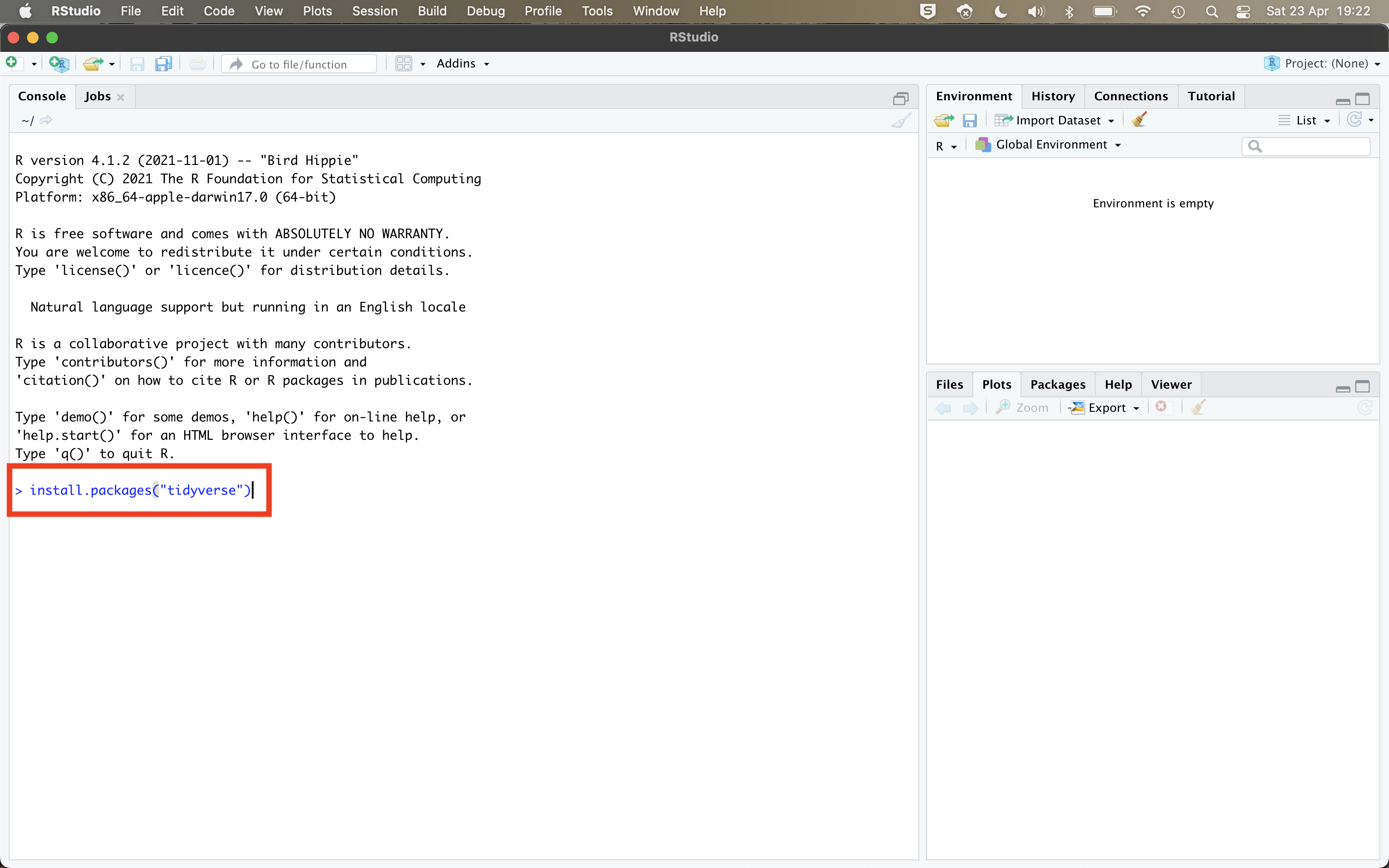
To install the tidyverse package from CRAN, you just type the following code into the Console and press Enter (see also the screenshot below):
install.packages("tidyverse")If you are connected to the internet, R will now download and install the package automatically. This might take a bit, and a lot of computer code gibberish will appear on your screen — no reason to worry, this is normal!
In some cases, R might ask you questions during the installation process (this applies to all package installations, now and in the future):
- If it asks you to update packages, choose “CRAN packages only” (press
2) - If it asks you whether you want to “install from sources that need compilation”, choose “No” (press
N)
(Did you by accident choose a wrong answer to one of the questions above? No worries, just re-run the install.packages("tidyverse") command above to start the installation process again.)
5.2 What you should see
If all worked out, your Console should say that “the downloaded binary packages are in…”, followed by some gibberish (see also the example screenshot below).
The result will look similar on a Windows computer (but with a bit more gibberish).
5.3 Installing the bst290 package
Next to the tidyverse package, we will also use a package that was specifically designed for this course: The bst290 package (see also github.com/cknotz/bst290). This package includes a small practice dataset and a few tools to easily create descriptive tables for your course assignments. It also includes an interactive dashboard that can help you understand the really tricky statistics-concepts we will cover in this course (the Central Limit Theorem, confidence intervals, statistical tests) better.
The bst290 package is not (yet) available from CRAN, but you can install it directly from GitHub. GitHub is a popular platform for computer programmers and researchers to share their code with others, and many R packages are distributed via GitHub.
Installing the bst290 package from GitHub involves two steps:
First, you need to install the remotes package — this is used to install packages from “remote” repositories like GitHub. You can install the remotes package directly from CRAN, just like with the tidyverse package earlier.
You type the following into the Console and press Enter:
install.packages("remotes")You will now see a lot more computer code gibberish running over your screen — again, nothing to worry about as long as you get the same result as earlier.
R might give you a warning that you should have something called RTools installed — this is not necessary for now! Just move on. If you want to install RTools anyways, you can do this in a few more steps. You can find an instruction here: https://cran.r-project.org/bin/windows/Rtools/rtools40.html.
Next, you use the remotes package to download and install the bst290 package from GitHub. To do so, type the following code into the Console and press Enter:
remotes::install_github("cknotz/bst290")This might again take a bit and you will probably again see a lot more computer gibberish appear — just hang in there. As before:
- If
Rasks you to update packages, choose “CRAN packages only” (press2) - If it asks you whether you want to “install from sources that need compilation”, choose “No” (press
N)
5.4 Installing the tinytex package
The third add-on package you need to install is called tinytex. tinytex is really nothing more than a tool to install the TinyTex software automatically through RStudio. You need to have TinyTex to be able to create PDF code reports for your assignments.3
You install tinytex just like the other packages:
install.packages("tinytex")Once that is complete, you run the following in your Console to install the TinyTex software:
tinytex::install_tinytex()The download and installation may take a few minutes – and there will be more code gibberish – so just hang in there!
You may get an error message that looks like this:
Found '/Library/TeX/texbin/tlmgr', which indicates a LaTeX distribution may have existed in the system.If that is the case, press N for No and cancel the installation. Most likely, you already have the necessary software installed to create PDF reports.
5.5 Loading packages
When you install a new app on your smartphone, it only gets installed but it does (usually) not open and run automatically. You as the user need to open it yourself.
This works similarly in R: Installing a package is Step 1 — you as the R user have to get active if you then want to use the new package.
5.5.1 Loading an entire package with library()
To load an installed package, you normally use the library() function. For example, to load the tidyverse package, you use:
library(tidyverse)When you run this code, you will get information about the packages that get loaded (“attached”). As mentioned, the tidyverse is a collection of packages. Therefore, if you load it, it loads a whole set of different packages: ggplot2 (for visualization), dplyr for data management, or stringr for working with text.
You will also be told about a number of conflicts. These conflicts are nothing to worry about, at least for now.4
You can load the bst290 package the same way:
library(bst290)There should now not be any warnings, etc.
You can also directly “call” specific functions from a package using the “double-colon” method: package::function(). You can use this directly, without loading the entire package first.
Maybe you notice that you already used that method earlier, when you installed the bst290 package: remotes::install_github(). In this case, you used just this one specific function from the remotes package.
6 Summary
Congrats! You have now:
- Installed
RandRStudio - Installed packages that we will use during this course
You can test if everything worked by running the following code in your Console:
bst290::practiceStatistics()This should open the dashboard from the bst290 package, and if this dashboard does indeed pop up on your screen then you are all set and ready to start the course!
Footnotes
See also the example job ads on Canvas (under “Why do I have to learn this?!”).↩︎
You can also always check where exactly your working directory currently is by using the
getwd()(“get working directory”) command. So, if you entergetwd()into the Console and press the Enter-key, you will be shown the file path to the folder that you are currently working in — where all your graphs, tables, etc. get put in when you export them fromR. You can also manually change your working directory withsetwd(). You just need to add a valid file path within the parentheses. For example, this would be file path that I could use on my own computer:setwd(""/Users/carloknotz/Documents/Work/Teaching/BST290/R_Tutorials").↩︎TinyTexis a small version of theLaTeXtypesetting software on your computer, whichRStudiothen uses to create the code reports (see also https://yihui.org/tinytex/).↩︎What this tells you is that there are certain commands (“functions”) in the packages you just loaded that have the same name as some other functions that are in use. For example,
dplyr::filter() masks stats::filter()means: “There is a function calledfilter()in thedplyrpackage that was just loaded. That function has the same name as anotherfilter()function, which is included in thestatspackage that comes withRright out of the box.dplyrwas loaded last, so if you now use thefilter()function, the one from thedplyrpackage will be used.”↩︎


