Tutorial 10: It depends! Interactive regression models

Introduction

Tutorials 8 and 9 showed you how you can estimate and interpret bi- and multivariate linear regression (OLS) models in R. The goal there was to figure out the effects of your independent (“explanatory”) variables on your dependent variable. A linear regression model shows you these effects in the form of coefficients: How does the dependent variable change when a given independent variable changes?

The previous analyses also treated each independent variable’s effect as separate: Education had its effect on political trust, which was separate from the effect of gender, and both of these effects were separate from the effect of age.

Treating effects as separate can make sense in many cases, but there are also situations when you may have reasons to expect that the strength or direction of the effect of one independent variable depends on another independent variable. For example, we often expect that gender can moderate the effect of an independent variable, meaning that the variable has an effect only for men but not for women (or vice versa). This type of effect or relationship where the effect of one variable depends on another is called interactive: Two variables interact with each other in producing a change in the dependent variable.

Accordingly, a regression model that includes an interaction between two independent variables is called an interactive regression model. This type of model is widely used in political and social research.¹

Specifying and estimating interactive models in R is not particularly difficult — but what is more difficult is the interpretation and presentation of the results. In the past, researchers often did not do this correctly, which led them to draw incorrect conclusions. But nowadays there is an established way of interpreting interaction effects by looking at marginal effects (or conditional effects), and there are packages for R that make calculating these marginal effects and presenting them fairly easy.² One of these is the margins package.

This tutorial will show you how you specify, interpret, and present interactive regression analyses. We continue with the case from earlier tutorials where we looked at trust in politicians using data from round 7 of the ESS.

Hypotheses

One of the results of the previous analyses was that people’s trust in politicians decreases as they get older. In other words, we found that age has a negative effect on trust in politicians. The effect was small, but statistically significant.

But remember also that we studied how men and women differ when it comes to political involvement. Specifically, one of the hypotheses we tested in a previous tutorial was that women are less politically active than men — or at least used to be in past decades.

If that last hypothesis is true, then we would expect that older generations today still carry the patterns from past times with them: Among older people, women tend to be less politically engaged. And this could mean that the negative effect of age on political trust exists only for men. Simply put, women in older generations have maybe always cared less about politics in general, and their getting older has therefore less of an effect on their trust in politicians than it has in the case of men.

The guiding hypothesis for this tutorial is therefore:

Gender conditions the negative effect of age on trust in politicians: The effect exists only for men, but not for women.

The corresponding null hypothesis is:

Gender has no conditioning effect: The negative effect of age on trust in politicians is the same for men and women.

Setup

The setup and data management part are almost exactly the same as in the previous tutorial, so this part will be very brief.

Packages

As before, we use the tidyverse to help with data management and visualization and texreg to make neat-looking regression tables.

library(tidyverse)
library(texreg)

But we now also need to load the margins package, which allows you to calculate marginal effect estimates. If you have not yet installed this package, you need to do so with install.packages("margins"). Once this is done, you load the package with library(). In addition, we will use the prediction package:

library(margins)
library(prediction)

Data import and data cleaning

This part is exactly as before and you should now already know what to do here (see Tutorials 8 and 9 for details):

1. Use haven::read_dta() to import the ESS round 7 (2014) dataset; save it as ess7
2. Transform the dataset into the familiar format using labelled:: unlabelled();
3. Trim the dataset:
   • Keep only observations from Norway;
   • Select the following variables: essround, idno, cntry, trstplt, eduyrs — and also agea, and gndr;
   • Use the pipe to link everything;
   • Save the trimmed dataset as ess7;
4. If you like, create a data dictionary using labelled::generate_dictionary();
5. Transform the trstplt variable from factor to numeric using as.numeric(); do not forget to adjust the scores; store the new variable as trstplt_num;
6. Drop the empty levels of the gndr variable with droplevels();

Interactive regression models

Models & formulas

In the previous two tutorials, we first estimated a bivariate regression model (which included only one independent variable) and then a multivariate regression model (which included three independent variables). Just to refresh your memory, the model equations looked like this:

The bivariate model included only a single independent variable (eduyrs) but no control variables:

\[\begin{align*} \texttt{trstplt\_num} = \alpha + \beta_1 \texttt{eduyrs} + \epsilon \end{align*}\]

The multivariate model then included also age (agea) and gender (gndr) as additional independent variables: \[\begin{align*} \texttt{trstplt\_num} = \alpha + \beta_1 \texttt{eduyrs} + \beta_2 \texttt{gndr} + \beta_3 \texttt{agea} + \epsilon \end{align*}\]

This last model assumes that all the independent variables work separately, that each has its own unique effect and this effect does not depend on the other variables. But the guiding hypothesis for this tutorial is of course that things depend: Specifically, that the effect of age depends on gender. This means we need to extend the multivariate model to let the effect of age vary by gender, which we do by including an interaction term.

To interact two variables, you multiply them. Specifically, you keep the two main variables in the model (plus any other additional controls) but then you also add a new term that is the product of the two constituent variables. In this case here, this would be the product of product of age and gender. If we add that interactive term, the model becomes an interactive regression model:

\[\begin{align*} \texttt{trstplt\_num} = \alpha + \beta_1 \texttt{eduyrs} + \beta_2 \texttt{gndr} + \beta_3 \texttt{agea} + \textcolor{blue}{\beta_4 (\texttt{gndr} \times \texttt{agea}}) + \epsilon \end{align*}\]

The results of this model now become much more difficult to interpret:

• The coefficient for gndr, \(\beta_2\) is now not the unique effect of gender but the effect of gender when agea is exactly 0 (and, by implication, the interaction term is also 0).
• Similarly, the coefficient for agea, \(\beta_3\) is no longer the unique effect of age but instead the effect of age when the gender-dummy is 0 (and, again, the interaction term is 0). Depending on how the gender-dummy is specified, this can be the case for men or women.
• The coefficient for the interaction term, \(\beta_4\) shows you how much the effects of age and gender vary: How much the effect of age differs between genders, but also how much the effect of gender differs by age.
• The coefficient for education, \(\beta_1\) is not part of the interaction. Therefore, you interpret it as before: The unique effect of an additional year of education on trust in politicians.

You probably notice that this is quite hard to wrap your head around — but this gets easier when we instead look at marginal effects, which comes below. First, however, we look at how you specify an interactive model in R.

Model specification in R

As you know, the formula for the multivariate model (with all control variables) would be written like this:

trstplt_num ~ eduyrs + gndr + agea

There are now two ways to make the model interactive. The first option is to extend the previous equation with the interactive term that multiplies agea with gndr (for which you use the colon-symbol):

trstplt_num ~ eduyrs + gndr + agea + gndr:agea

A simpler (but more indirect) way is to directly interact gndr with agea with the multiplication symbol. R will then automatically add individual terms for agea and gndr plus the interactive term when it runs the calculation:

trstplt_num ~ eduyrs + gndr*agea

Estimating interactive models with lm()

To start, we quickly re-estimate the bi- and multivariate models from the previous tutorials so that we can compare these results to the interactive model’s results (and because you should anyways proceed in this stepwise fashion):³

# bivariate model
model1 <- lm(trstplt_num ~ eduyrs, 
             data = ess7)

# multivariate model
model2 <- lm(trstplt_num ~ eduyrs + gndr + agea, 
             data = ess7)

Now that we have these models as a baseline comparison, we estimate the interactive model and print a quick summary of the results to the Console:

# interactive model
model3 <- lm(trstplt_num ~ eduyrs + gndr*agea, 
             data = ess7)
summary(model3)

Call:
lm(formula = trstplt_num ~ eduyrs + gndr * agea, data = ess7)

Residuals:
   Min     1Q Median     3Q    Max 
-5.867 -1.192  0.206  1.435  5.064 

Coefficients:
                 Estimate Std. Error t value Pr(>|t|)    
(Intercept)      4.813994   0.271636  17.722  < 2e-16 ***
eduyrs           0.070857   0.013885   5.103 3.79e-07 ***
gndrFemale      -0.389786   0.277113  -1.407  0.15977    
agea            -0.012221   0.003797  -3.219  0.00132 ** 
gndrFemale:agea  0.009818   0.005488   1.789  0.07382 .  
---
Signif. codes:  0 '***' 0.001 '**' 0.01 '*' 0.05 '.' 0.1 ' ' 1

Residual standard error: 1.927 on 1422 degrees of freedom
  (9 observations deleted due to missingness)
Multiple R-squared:  0.02745,   Adjusted R-squared:  0.02471 
F-statistic: 10.03 on 4 and 1422 DF,  p-value: 5.234e-08

When you look at the summary, you can directly see that R has automatically “populated” the model with the correct terms: An individual term for eduyrs, then a dummy for women using gndr, another term for agea, and finally the interaction term between agea and gndrFemale (gndrFemale:agea).

You can see already here that the interaction term is at least significant at the 10% level (indicated by the single dot in the last line). So there might be something there. But to really know, we need to look at marginal effects.

Before that, we first print all the results in a proper table:

screenreg(list(model1,model2,model3),
          custom.coef.names = c("Intercept",
                                "Years of educ. completed",
                                "Female",
                                "Age",
                                "Female x Age"),
          custom.model.names = c("Bivariate",
                                 "Multivariate",
                                 "Interactive"),
          stars = 0.05)

==============================================================
                          Bivariate  Multivariate  Interactive
--------------------------------------------------------------
Intercept                    4.23 *     4.62 *        4.81 *  
                            (0.20)     (0.25)        (0.27)   
Years of educ. completed     0.07 *     0.07 *        0.07 *  
                            (0.01)     (0.01)        (0.01)   
Female                                  0.07         -0.39    
                                       (0.10)        (0.28)   
Age                                    -0.01 *       -0.01 *  
                                       (0.00)        (0.00)   
Female x Age                                          0.01    
                                                     (0.01)   
--------------------------------------------------------------
R^2                          0.02       0.03          0.03    
Adj. R^2                     0.02       0.02          0.02    
Num. obs.                 1427       1427          1427       
==============================================================
* p < 0.05

Calculating, presenting, and interpreting marginal effects

Basic use

Now to the interesting part where we really make sense of the model results by looking at marginal effects. Marginal effects are more meaningful and easy to understand because they tell us the overall effect of one variable at different levels of another one: E.g., what is the effect of age for women and then for men?

R, or more specifically the margins-package can calculate marginal effects from the ‘raw’ model results via the margins() function. This function works like this:

1. You need to specify the model that you want the calculation to be based on. In this case, this would be model3.
2. You need to specify for which variable you want marginal effects calculated. In this case, this would be agea.
3. You need to specify over which other variable these marginal effects should vary. Here, this would be gndr.

Putting it all together, the complete margins() call would look like this:

margins(model = model3,
        variables = "agea",
        at = list(gndr = c("Female","Male")))

 at(gndr)      agea
     Male -0.012221
   Female -0.002403

These numbers may seem cryptic at first sight, but they are actually relatively easy to read. The first line gives you the effect of age for women. You read this as: If someone is a woman, every additional year of age decreases trust in politicians by a very tiny -0.002 points.

The second line gives you the corresponding result for men: If someone is a man, every additional year of age decreases trust in politicians by -0.012 points.

In both cases, the effects are surely not very large — but you also see that the effect of age for men, however small it may be, is still about five times as large as the tiny effect for women (-0.012221/-0.002403 = 5.085726). So, it does look like the effect of age differs by gender!

Getting p-values and confidence intervals

The results we have so far are interesting, but they are only half of the story — we also need to account for the fact that these numbers are estimates based on sample data and that we cannot just take them at face value. We also need to look if they really are statistically significant, meaning if we can say with sufficient confidence that these effects also exist in the general population for which we want to make inferences. As you know, we look at p-values and confidence intervals to figure this out.

To get these additional statistics, we use margins()’s sister-function, margins_nummary():

margins_summary(model = model3, 
                variables = "agea", 
                at = list(gndr = c("Male","Female")))
 factor   gndr     AME     SE       z      p   lower   upper
   agea 1.0000 -0.0122 0.0038 -3.2186 0.0013 -0.0197 -0.0048
   agea 2.0000 -0.0024 0.0040 -0.6039 0.5459 -0.0102  0.0054

This result now tells us the complete story, only the values of the gndr variable are presented in a less informative way. But we can simply use bst::visfactor() to figure out what 1 and 2 correspond to:

bst290::visfactor(variable = "gndr", dataset = ess7)
 values labels
      1   Male
      2 Female

If we now look at the margins_summary() result and specifically at the p-values (under p), we see that only the marginal effect of age for men (see AME) is really statistically significant (p = 0.0013 < 0.05). The marginal effect of age for women, on the other hand, is not (p = 0.5459).

This means: There (probably) is a small negative effect of age on trust in politicians in the general Norwegian population — but this effect exists only among Norwegian men. In the case of women, we cannot say with sufficient confidence if the true effect is really different from 0 or not, and so we assume that age has no effect on political trust in the case of Norwegian women.

You can also see this if you look at the last two columns of the result, which give you the upper and lower limits of the confidence intervals of the marginal effect estimates. The confidence interval for men does not include 0, while the one for women does overlap with 0.

Visualizing marginal effect estimates

To make the interpretation of the results still more intuitive for yourself (and especially for your readers!), you can and should visualize the result. Luckily, the output you get from margins_summary() is a data.frame, which means you can directly “pipe” it into a ggplot() graph.

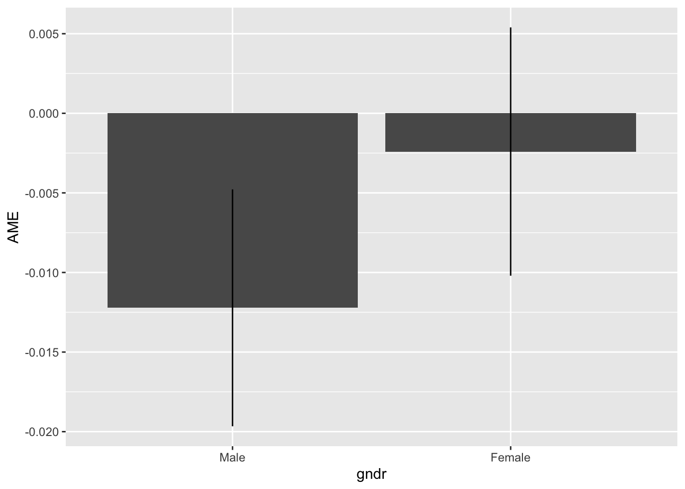
A raw, unpolished graph (here a bar graph; geom_point() is an alternative) would look like this:

margins_summary(model = model3, 
                variables = "agea", 
                at = list(gndr = c("Male","Female"))) %>% 
  ggplot(aes(x = gndr, y = AME, ymin = lower, ymax = upper)) +
    geom_bar(stat = "identity") + # draws marginal effect estimates as bars
    geom_linerange() # draws confidence intervals as lines

Note that geom_linerange(), which draws the confidence intervals, needs to know the upper and lower values of the lines it is supposed to draw. You need to specify these with ymin and ymax within aes().

What you see here are the marginal effect estimates of age separately for men and women. You can directly see that the effect of age is more strongly negative for men than for women. If you look carefully, you can also see that the confidence interval overlaps with 0 in the case of women — indicating again the lack of statistical significance.

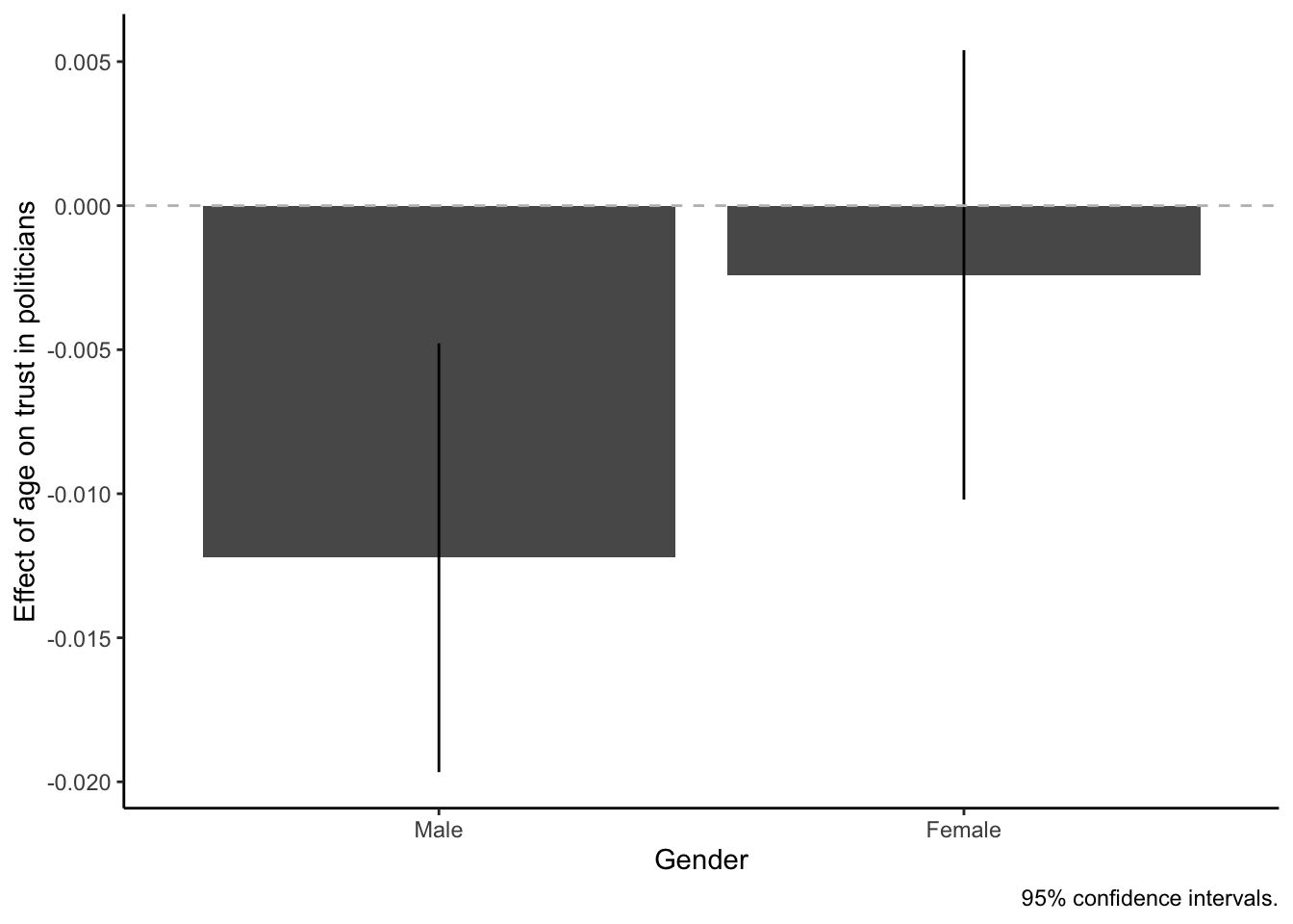
To make the interpretation even easier, we would polish the graph a bit more by adding proper labels to the axes, using a better-looking scheme, and also by adding a horizontal reference line at the 0-point on the y-axis with geom_hline().

margins_summary(model = model3, 
                variables = "agea", 
                at = list(gndr = c("Male","Female"))) %>% 
  ggplot(aes(x = gndr, y = AME, ymin = lower, ymax = upper)) +
    geom_bar(stat = "identity") +
    geom_linerange() +
    geom_hline(yintercept = 0, linetype = "dashed", color = "gray") +
    labs(x = "Gender",
         y = "Effect of age on trust in politicians",
         caption = "95% confidence intervals.") +
    theme_classic()

This graph should make the overall result fairly apparent: Among men, every additional year of age decreases trust in politicians by around -0.012 points. Among women, on the other hand, the effect of age is not significantly different from 0. In other words, we have shown that the effect of age on trust in politicians depends on gender! Only men trust politicians less as they get older, while age makes no difference for women.

Predictions

A second way to interpret the results of an interactive regression model is to calculate and visualize predicted outcomes. In this case, it would be interesting to look at how trust in politicians changes as people get older, and how that differs between men and women.

You may already have guessed that we will now use the prediction package. Specifically, we will use its prediction_summary() function to calculate predicted trust scores over values of agea and gndr. The logic of the code to do this is very similar to that used with margins():

prediction_summary(model = model3,
                   at = list(gndr = c("Male","Female"),
                             agea = seq(from = 20, to = 75, by = 5)))

 at(gndr) at(agea) Prediction      SE     z          p lower upper
     Male       20      5.551 0.12148 45.69  0.000e+00 5.313 5.789
   Female       20      5.357 0.13260 40.40  0.000e+00 5.097 5.617
     Male       25      5.490 0.10654 51.53  0.000e+00 5.281 5.698
   Female       25      5.345 0.11669 45.81  0.000e+00 5.117 5.574
     Male       30      5.429 0.09307 58.33  0.000e+00 5.246 5.611
   Female       30      5.333 0.10218 52.20  0.000e+00 5.133 5.534
     Male       35      5.367 0.08183 65.59  0.000e+00 5.207 5.528
   Female       35      5.321 0.08976 59.29  0.000e+00 5.145 5.497
     Male       40      5.306 0.07383 71.87  0.000e+00 5.162 5.451
   Female       40      5.309 0.08040 66.03  0.000e+00 5.152 5.467
     Male       45      5.245 0.07019 74.73  0.000e+00 5.108 5.383
   Female       45      5.297 0.07526 70.38  0.000e+00 5.150 5.445
     Male       50      5.184 0.07157 72.43  0.000e+00 5.044 5.324
   Female       50      5.285 0.07521 70.27  0.000e+00 5.138 5.433
     Male       55      5.123 0.07771 65.92  0.000e+00 4.971 5.275
   Female       55      5.273 0.08025 65.71  0.000e+00 5.116 5.431
     Male       60      5.062 0.08762 57.77  0.000e+00 4.890 5.234
   Female       60      5.261 0.08954 58.76  0.000e+00 5.086 5.437
     Male       65      5.001 0.10018 49.92  0.000e+00 4.804 5.197
   Female       65      5.249 0.10191 51.51  0.000e+00 5.049 5.449
     Male       70      4.940 0.11452 43.13  0.000e+00 4.715 5.164
   Female       70      5.237 0.11638 45.00  0.000e+00 5.009 5.465
     Male       75      4.879 0.13006 37.51 6.187e-308 4.624 5.134
   Female       75      5.225 0.13227 39.50  0.000e+00 4.966 5.484

In this case, we ask for predicted scores for ages from 20 to 75 in steps of 5 years, and this separately for men and for women.

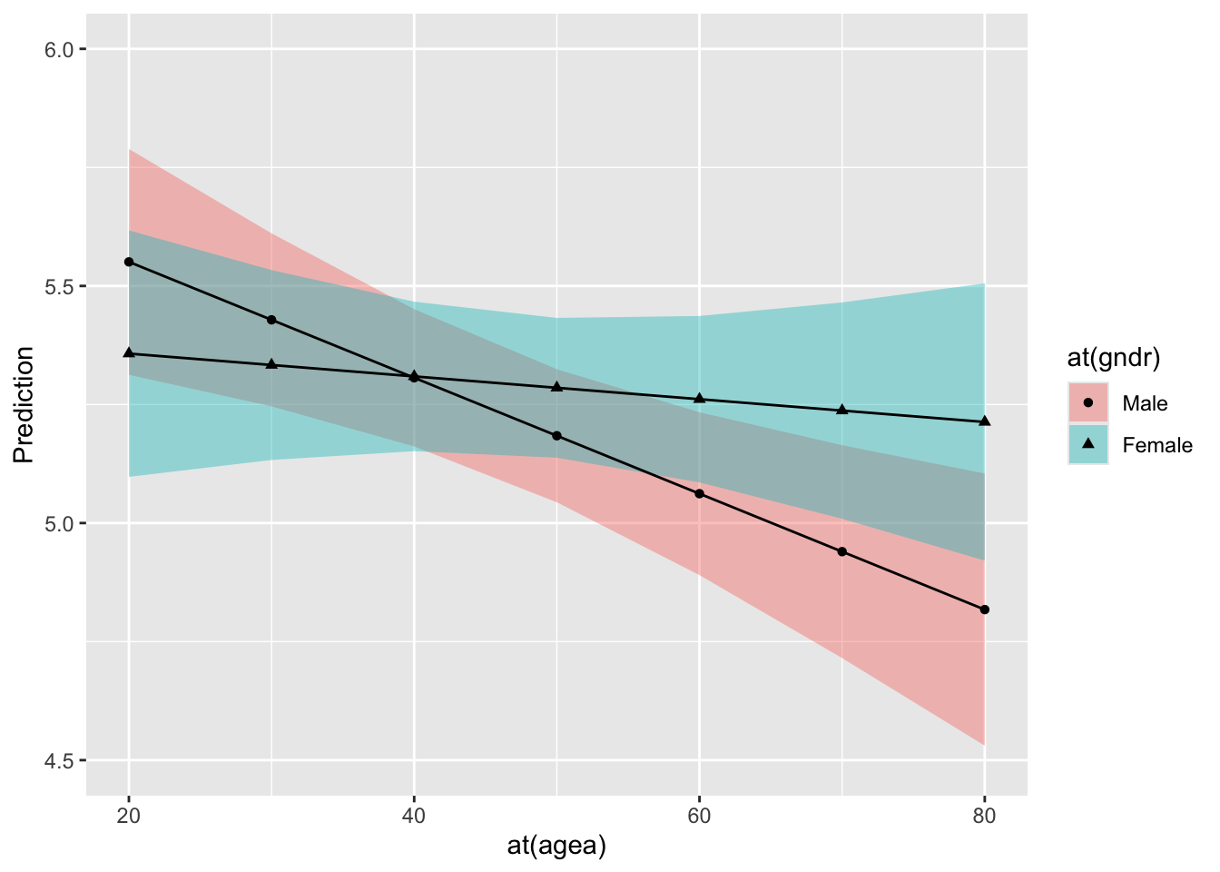
The result contains lots and lots of numbers, and any patterns in it will be more easily visible when visualized:

prediction_summary(model = model3,
                   at = list(gndr = c("Male","Female"),
                             agea = seq(from = 20, to = 80, by = 10))) %>% 
  ggplot(aes(x = `at(agea)`, y = Prediction,fill = `at(gndr)`,
             shape = `at(gndr)`, ymin = lower, ymax = upper)) +
    geom_ribbon(alpha = .4) +
    geom_point() +
    geom_line() +
    scale_y_continuous(breaks = seq(from = 4.5, to = 6, by = .5),
                       limits = c(4.5,6)) # this adjust the range and labels of the y-axis

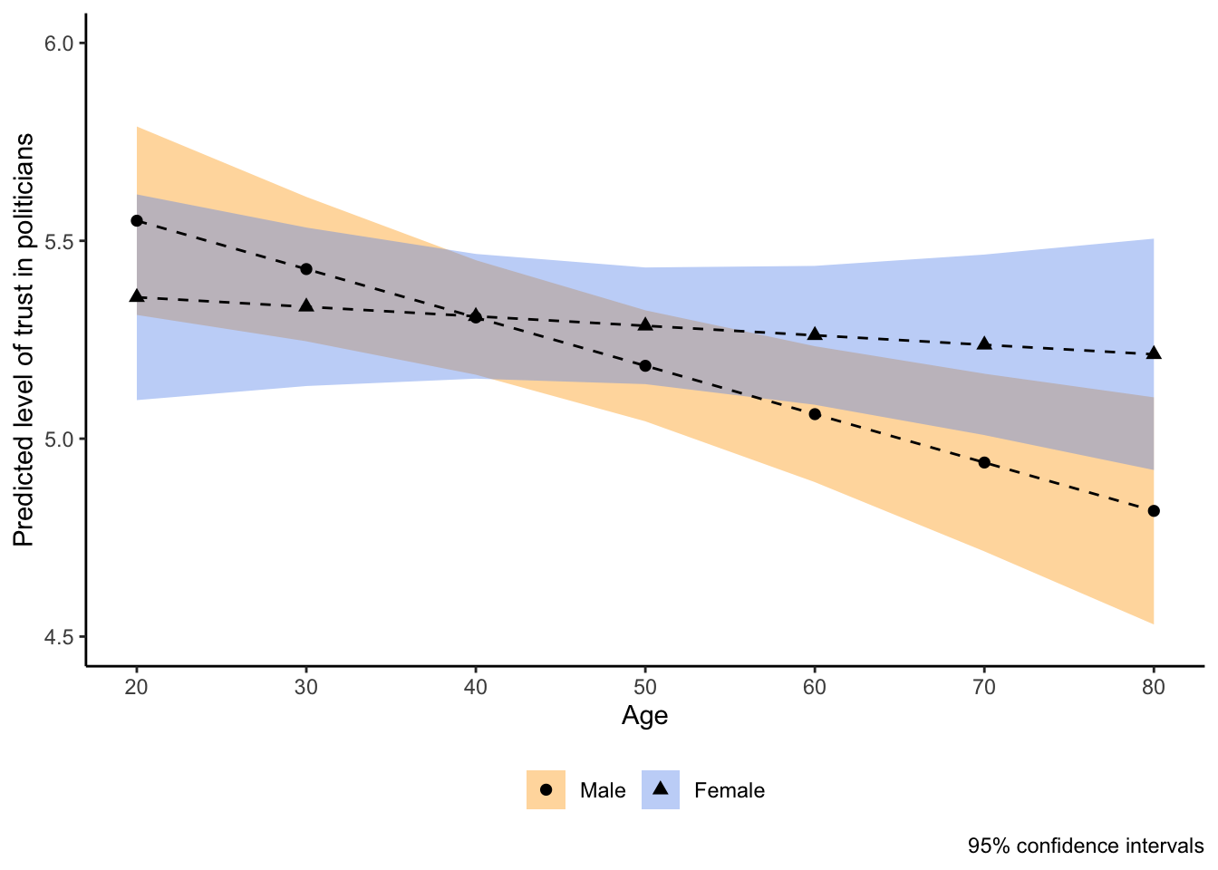
You can see that as women get older, their level of trust barely changes. For men, on the other hand, there is a more pronounced decrease over time. Of course, the change is substantively small – as you can also see when you look at the range of the y-axis.

With some more polishing, we end up with a nice and informative graph about the conditional effect of age on political trust:

prediction_summary(model = model3,
                   at = list(gndr = c("Male","Female"),
                             agea = seq(from = 20, to = 80, by = 10))) %>% 
  ggplot(aes(x = `at(agea)`, y = Prediction,fill = `at(gndr)`,
             shape = `at(gndr)`, ymin = lower, ymax = upper)) +
    geom_ribbon(alpha = .4) +
    geom_point(size = 2) +
    geom_line(linetype = "dashed") +
    scale_y_continuous(breaks = seq(from = 4.5, to = 6, by = .5),
                       limits = c(4.5,6)) + 
    scale_x_continuous(breaks = seq(from = 20, to = 80, by = 10),
                       limits = c(20,80)) +
    scale_fill_manual(values = c("Orange","Cornflowerblue")) +
    labs(x = "Age", y = "Predicted level of trust in politicians",
         caption = "95% confidence intervals") +
    theme_classic() +
    theme(legend.position = "bottom", # move legend to bottom
          legend.title = element_blank()) # remove legend title

Footnotes

1. For example, Liechti et al. (Liechti, F., Fossati, F., Bonoli, G., and Auer, D. (2017). The signalling value of labour market programmes. European Sociological Review, 33(2):257–274.) show that labor market re-integration programs for unemployed workers have different effects depending on whether the unemployed worker is an immigrant or not.

2. A widely-cited studied that established this (and which you should cite if you estimate interactive models) is Brambor, T., Clark, W. R., and Golder, M. (2006). Understanding interaction models: Improving empirical analyses. Political Analysis, 14(1):63–82.

3. See Lenz, G. S. and Sahn, A. (2021). Achieving statistical significance with control variables and without transparency. Political Analysis, 29(3):356–369.