Tutorial 9: Multivariate linear regression

1 Introduction

In the previous tutorial, you learned how to estimate a bivariate linear regression model in R. You used a linear regression model to see if people’s level of education influences their level of trust in politicians. The expectation was that higher education would lead to greater trust in politicians, and that is also what we found.

In this tutorial, we go one step further and test if this bivariate relationship stays the same (“is robust”) when we control for additional factors. We do so by estimating a multivariate regression model. In this type of model, we estimate the effects of several independent variables (predictors) on a dependent variable simultaneously.

Tip

Hvis du ønsker å lese en norsk tekst i tillegg: “Lær deg R”, Kapittel 8.

2 Setup

2.1 Packages, data import, and first data cleaning

As before, we use the tidyverse to help with data management and visualization and texreg to make neat-looking regression tables.

library(tidyverse)
library(texreg)

You should now already know what to do next, and how to do it:

1. Use haven::read_dta() to import the ESS round 7 (2014) dataset; save it as ess7;
2. Transform the dataset into the familiar format using labelled::unlabelled();
3. Trim the dataset:
   • Keep only observations from Norway;
   • Select the following variables: essround, idno, cntry, trstplt, eduyrs — and also agea, and gndr;
   • Use the pipe to link everything;
   • Save the trimmed dataset as ess7;
4. If you like, create a data dictionary using labelled::generate_dictionary();
5. Transform the trstplt variable from factor to numeric using as.numeric(); do not forget to adjust the scores; store the new variable as trstplt_num;

2.2 New data management: additional independent variables

In addition to the main predictor from the previous tutorial (eduyrs, the respondent’s level of education), we want to add controls for two additional variables:

• The respondent’s age in years, using agea
• The respondent’s gender, using gndr

We take a quick look at how these variables are stored:

class(ess7$agea)
[1] "numeric"
class(ess7$gndr)
[1] "factor"

Luckily, these variables are stored correctly: agea is numeric, and gndr is a factor — as they should be.

3 (New) descriptive statistics

As before, we print out some descriptive statistics for our variables. It is important to report these so that readers get an idea of how our data look like and can interpret the results correctly.

To report statistics for our numeric variables, we simply expand the descriptive table we created in the previous tutorial:

bst290::oppsumtabell(dataset = ess7,
                     variables = c("trstplt_num","agea","eduyrs"))
 Variable        trstplt_num agea    eduyrs 
 Observations    1429.00     1436.00 1434.00
 Average            5.26       46.77   13.85
 25th percentile    4.00       32.00   11.00
 Median             5.00       47.00   14.00
 75th percentile    7.00       61.25   17.00
 Stand. Dev.        1.95       18.68    3.72
 Minimum            0.00       15.00    0.00
 Maximum           10.00      104.00   30.00
 Missing            7.00        0.00    2.00

The gender-variable is not numeric, so including it in the summary table is not recommended. But you can report its distribution using a simple bar graph:

ess7 %>% 
  ggplot(aes(x = gndr)) +
    geom_bar() +
    labs(x = "Respondent's gender",
         y = "Number of observations") +
    theme_bw()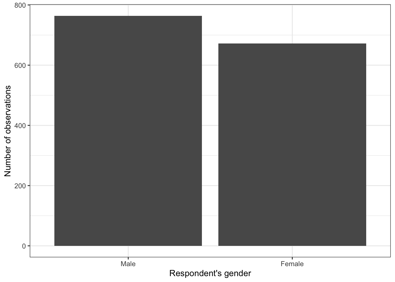

Alternatively, you could also create a simple table with table():

table(ess7$gndr)

  Male Female 
   764    672 

4 Regression analysis

4.0.1 Models & formulas (again)

Recall the formula for the bivariate regression model we estimated in the last tutorial. This model included only a single independent variable (eduyrs) but no control variables:

\[\begin{align*} \texttt{trstplt\_num} = \alpha + \beta_1 \texttt{eduyrs} + \epsilon \end{align*}\]

Now we expand this model by adding more independent variables — the model becomes multivariate: \[\begin{align*} \texttt{trstplt\_num} = \alpha + \beta_1 \texttt{eduyrs} + \beta_2 \texttt{gndr} + \beta_3 \texttt{agea} + \epsilon \end{align*}\]

As before:

• \(\alpha\) is still the intercept (konstantledd).
• The \(\beta\)s are the regression coefficients (or “weights”, stigningstall).
• \(\epsilon\) is still the error term.

In R, the formula for the multivariate model (with all control variables) would be written like this:

trstplt_num ~ eduyrs + gndr + agea

As before, R takes care of the intercept and the error term — all we have to do to get a multivariate regression model is to list more than one independent variable. Easy.

4.1 The lm() function

Just to refresh your memory, we first estimate the bivariate regression model from the previous tutorial and store the result as model1:

model1 <- lm(trstplt_num ~ eduyrs, 
             data = ess7)

If you like, you can also print out the result with summary():

summary(model1)

Call:
lm(formula = trstplt_num ~ eduyrs, data = ess7)

Residuals:
    Min      1Q  Median      3Q     Max 
-5.7148 -1.1966  0.0996  1.4332  5.0256 

Coefficients:
            Estimate Std. Error t value Pr(>|t|)    
(Intercept)  4.23401    0.19737  21.452  < 2e-16 ***
eduyrs       0.07404    0.01377   5.378 8.78e-08 ***
---
Signif. codes:  0 '***' 0.001 '**' 0.01 '*' 0.05 '.' 0.1 ' ' 1

Residual standard error: 1.932 on 1425 degrees of freedom
  (9 observations deleted due to missingness)
Multiple R-squared:  0.0199,    Adjusted R-squared:  0.01921 
F-statistic: 28.93 on 1 and 1425 DF,  p-value: 8.779e-08

In the next step, we test if the effect of eduyrs is robust to including the additional control variables: gender and age.

This means that we estimate our multivariate model, store the result as model2, and print out the results:

model2 <- lm(trstplt_num ~ eduyrs + gndr + agea, data = ess7)
summary(model2)

Call:
lm(formula = trstplt_num ~ eduyrs + gndr + agea, data = ess7)

Residuals:
    Min      1Q  Median      3Q     Max 
-5.7539 -1.1985  0.1983  1.4072  5.2348 

Coefficients:
             Estimate Std. Error t value Pr(>|t|)    
(Intercept)  4.621764   0.249674  18.511  < 2e-16 ***
eduyrs       0.069118   0.013861   4.986 6.91e-07 ***
gndrFemale   0.070814   0.102590   0.690  0.49014    
agea        -0.007544   0.002756  -2.737  0.00627 ** 
---
Signif. codes:  0 '***' 0.001 '**' 0.01 '*' 0.05 '.' 0.1 ' ' 1

Residual standard error: 1.928 on 1423 degrees of freedom
  (9 observations deleted due to missingness)
Multiple R-squared:  0.02526,   Adjusted R-squared:  0.0232 
F-statistic: 12.29 on 3 and 1423 DF,  p-value: 6.121e-08

You see that the output looks the same as before, just with more coefficients listed. Notice also that R has automatically figured out that gndr is a factor variable and included a dummy only for women (gndrFemale) into the model (as also explained in Kellstedt & Whitten, Chapter 11.2).

Now it gets tricky: How do you make sense of these results? Kellstedt & Whitten (2018, Chapters 10 & 11) or Solbakken (Statistikk for Nybeginnere, Chapters 6 & 8) explain this.

4.2 Presenting the regression results in a publication-quality table

To present the results and export them as a nice-looking table, we use again the texreg package.

First, we print out a preview of our table using the screenreg() function. Now we have two regression models to print, so we have to list both in the function:

screenreg(list(model1, model2))

=====================================
             Model 1      Model 2    
-------------------------------------
(Intercept)     4.23 ***     4.62 ***
               (0.20)       (0.25)   
eduyrs          0.07 ***     0.07 ***
               (0.01)       (0.01)   
gndrFemale                   0.07    
                            (0.10)   
agea                        -0.01 ** 
                            (0.00)   
-------------------------------------
R^2             0.02         0.03    
Adj. R^2        0.02         0.02    
Num. obs.    1427         1427       
=====================================
*** p < 0.001; ** p < 0.01; * p < 0.05

When you look at the table, you can directly see the differences between the two models. Model 1 included only the intercept and education (eduyrs), while model 2 also included age and gender as control variables. The table includes all the variables’ coefficients: You see, for instance, the coefficients for education and how they differ (or not) between the two models.

Next, we add proper labels for the coefficients and trim the significance stars:

screenreg(list(model1,model2),
          custom.coef.names = c("Intercept",
                                "Years of educ. completed",
                                "Female",
                                "Age"),
          stars = 0.05)

==============================================
                          Model 1    Model 2  
----------------------------------------------
Intercept                    4.23 *     4.62 *
                            (0.20)     (0.25) 
Years of educ. completed     0.07 *     0.07 *
                            (0.01)     (0.01) 
Female                                  0.07  
                                       (0.10) 
Age                                    -0.01 *
                                       (0.00) 
----------------------------------------------
R^2                          0.02       0.03  
Adj. R^2                     0.02       0.02  
Num. obs.                 1427       1427     
==============================================
* p < 0.05

Finally, we use the wordreg() function to export the table to a Microsoft Word document:

wordreg(list(model1,model2),
          custom.coef.names = c("Intercept",
                                "Years of educ. completed",
                                "Female",
                                "Age"),
          stars = 0.05,
        file = "ols_models.doc")

5 Conclusion

Now you know how to estimate, interpret, and present a multivariate linear regression model in R. This opens a lot of doors, because you can now use data such as those from the ESS to really disentangle the drivers and determinants of complex social and political phenomena. Also, if you read political science and sociological research, you will find many, many publications that use this type of method, so you now have first-hand knowledge of what is behind the results that are presented there.

You can again find an interactive tutorial to practice working with linear regression models a bit more — by continuing the earlier analysis on why some people are happier than others.

References

Kellstedt, Paul M, and Guy D Whitten. 2018. The Fundamentals of Political Science Research. Cambridge University Press.
Solbakken, Simen Sørbøe. 2019. Statistikk for Nybegynnere. Fagbokforlaget.